JEE Main & Advanced Mathematics Probability Binomial Distribution

(1) Geometrical method for probability : When the number of points in the sample space is infinite, it becomes difficult to apply classical definition of probability. For instance, if we are interested to find the probability that a point selected at random from the interval [1, 6] lies either in the interval [1, 2] or [5, 6], we cannot apply the classical definition of probability. In this case we define the probability as follows:

\[P\{x\in A\}=\frac{\text{Measure of region }A}{\text{Measure of the sample space }S}\]

where measure stands for length, area or volume depending upon whether S is a one-dimensional, two-dimensional or three-dimensional region.

(2) Probability distribution : Let S be a sample space. A random variable X is a function from the set S to R, the set of real numbers.

For example, the sample space for a throw of a pair of dice is

\[S=\begin{matrix} \{11, & 12, & \cdots , & 16  \\ 21, & 22, & \cdots , & 26  \\ \vdots  & \vdots  & \ddots  & \vdots   \\ 61, & 62, & \cdots , & 66\}  \\ \end{matrix}\]

Let X be the sum of numbers on the dice. Then \[X(12)=3,\,X(43)=7\], etc. Also, \[\{X=7\}\] is the event \[\{61,\text{ }52,\text{ }43,\text{ }34,\text{ }25,\text{ }16\}\]. In general, if X is a random variable defined on the sample space S and r is a real number, then \[\{X=r\}\] is an event.

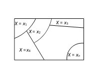
If the random variable X takes n distinct values \[{{x}_{1}},\,{{x}_{2}},\,....,\,{{x}_{n}}\], then \[\{X={{x}_{1}}\}\], \[\{X={{x}_{2}}\},\,....,\,\{X={{x}_{n}}\}\] are mutually exclusive and exhaustive events.

Now, since \[(X={{x}_{i}})\] is an event, we can talk of \[P(X={{x}_{i}})\]. If \[P(X={{x}_{i}})={{P}_{i}}\,(1\le i\le n)\], then the system of numbers.

\[\left( \begin{matrix}{{x}_{1}} & {{x}_{2}} & \cdots  & {{x}_{n}}  \\{{p}_{1}} & {{p}_{2}} & \cdots  & {{p}_{n}}  \\\end{matrix} \right)\]  is said to be the probability distribution of the random variable X.

The expectation (mean) of the random variable X is defined as \[E(X)=\sum\limits_{i=1}^{n}{{{p}_{i}}{{x}_{i}}}\]and the variance of X is defined as \[\operatorname{var}(X)=\sum\limits_{i=1}^{n}{{{p}_{i}}{{({{x}_{i}}-E(X))}^{2}}}=\sum\limits_{i=1}^{n}{{{p}_{i}}x_{i}^{2}-{{(E(X))}^{2}}}\] .

(3) Binomial probability distribution : A random variable X which takes values \[0,\text{ }1,\text{ }2,\text{ }\ldots ,n\] is said to follow binomial distribution if its probability distribution function is given by \[P(X=r)={{\,}^{n}}{{C}_{r}}{{p}^{r}}{{q}^{n-r}},\,r=0,\,1,\,2,\,.....,\,n\] where \[p,\,\,q>0\] such that \[p+q=1\].

The notation \[X\tilde{\ }B\,(n,\,\,p)\] is generally used to denote that the random variable X follows binomial distribution with parameters n and p.

We have \[P(X=0)+P(X=1)+...+P(X=n)\].

\[={{\,}^{n}}{{C}_{0}}{{p}^{0}}{{q}^{n-0}}+{{\,}^{n}}{{C}_{1}}{{p}^{1}}{{q}^{n-1}}+...+{{\,}^{n}}{{C}_{n}}{{p}^{n}}{{q}^{n-n}}={{(q+p)}^{n}}={{1}^{n}}=1\]

Now probability of

(a) Occurrence of the event exactly r times  \[P(X=r)={{\,}^{n}}{{C}_{r}}{{q}^{n-r}}{{p}^{r}}\].

(b) Occurrence of the event at least r times \[P(X\ge r)={{\,}^{n}}{{C}_{r}}{{q}^{n-r}}{{p}^{r}}+...+{{p}^{n}}=\sum\limits_{X=r}^{n}{^{n}{{C}_{X}}{{p}^{X}}{{q}^{n-X}}}\].

(c) Occurrence of the event at the most r times \[P(0\le X\le r)={{q}^{n}}+{{\,}^{n}}{{C}_{1}}{{q}^{n-1}}p+...+{{\,}^{n}}{{C}_{r}}{{q}^{n-r}}{{p}^{r}}=\sum\limits_{X=0}^{r}{{{p}^{X}}{{q}^{n-X}}}\].

• If the probability of happening of an event in one trial be p, then the probability of successive happening of that event in r trials is \[{{p}^{r}}\].

• If n trials constitute an experiment and the experiment is repeated N times, then the frequencies of \[0,\text{ }1,\text{ }2,\text{ }\ldots ,n\] successes are given by \[N.P(X=0),\,N.P(X=1),\,N.P(X=2),\,....,\,N.P(X=n)\].

(i) Mean and variance of the binomial distribution

The binomial probability distribution is

\[\begin{align}& \,\,\,X\,\,\,\,\,\,\,\,\,\,0\,\,\,\,\,\,\,\,\,\,\,\,\,\,\,\,\,\,1\,\,\,\,\,\,\,\,\,\,\,\,\,\,\,\,\,\,2\,\,\,\,\,\,\,.....\,\,\,\,\,\,\,\,\,n \\& P(X)\,\,{{\,}^{n}}{{C}_{0}}{{q}^{n}}{{p}^{0}}\,\,\,{{\,}^{n}}{{C}_{1}}{{q}^{n-1}}p\,\,{{\,}^{n}}{{C}_{2}}{{q}^{n-2}}{{p}^{2}}{{.....}^{n}}{{C}_{n}}{{q}^{0}}{{p}^{n}} \\\end{align}\]

The mean of this distribution is

\[\sum\limits_{i=1}^{n}{{{X}_{i}}{{p}_{i}}}=\sum\limits_{X=1}^{n}{X.{{\,}^{n}}{{C}_{X}}{{q}^{n-X}}{{p}^{X}}=np}\], 

The variance of the Binomial distribution is \[{{\sigma }^{2}}=npq\] and the standard deviation is \[\sigma =\sqrt{(npq)}\].

(ii) Use of multinomial expansion : If a die has m faces marked with the numbers \[1,\text{ }2,\text{ }3,\text{ }\ldots .\,\,m\] and if such n dice are thrown, then the probability that the sum of the numbers exhibited on the upper faces equal to p is given by the coefficient of \[{{x}^{p}}\] in the expansion of \[\frac{{{(x+{{x}^{2}}+{{x}^{3}}+....+{{x}^{m}})}^{n}}}{{{m}^{n}}}\].

(4) The poisson distribution : Let X be  a discrete random variable which can take on the values 0, 1, 2,... such that the probability function of X is given by \[f(x)=P(X=x)=\frac{{{\lambda }^{x}}{{e}^{-\lambda }}}{x!}\],  \[x=0,1,2,....\] where \[\lambda \] is a given positive constant. This distribution is called the Poisson distribution and a random variable having this distribution is said to be Poisson distributed.