Current Affairs 12th Class

                                                                                         Application of Derivatives    
  • Continuity and Differentiability of a function: Let a function \[y=f(x)\] is said to be continuous at
\[x=a\] then \[\underset{x\to {{a}^{-}}}{\mathop{\lim }}\,f(x)=\underset{x\to {{a}^{+}}}{\mathop{\lim }}\,\,\,f(x)=f(a)\] Generally, a function is said to be continuous at \[x=a\] when the graph of that function can be drawn/sketched without lefting the pencil.    
  • Differentiation: The process of finding out the differentiability/derivatives of the function \[y=f(x)\]in the interval (a, b) is said to be differentiation.
 
  • Derivatives of f(x): Let \[y=f(x)\] is continuous in interval [a, b]. Let a point \[c\in (a,b)\]
Then function \[y=f(x)\] is differentiable at \[x=c\] i.e. \[\underset{x\to c}{\mathop{\lim }}\,\frac{f(x+c)-(c)}{c}=f'(c)\]   Solved Example
  • Find derivative of \[y=\sin x.\] by 1st principle:
  • Let \[y=f(x)=\sin x\]    ...(1) Let \[\delta \]x be the small increment in x then \[\delta \]y be the corresponding increment in y. \[y+\delta y=\sin (x+\delta x)\]   ...(2) Now, on subtracting equation (1) from (2), we get \[y+\delta y-y=\sin (x+\delta x)-\sin x\] \[\delta y=2.\cos \frac{x+\delta x+x}{2}.\sin \left( \frac{x+\delta x+x}{2} \right)\] Dividing \[\delta \]x on both sides and taking limit \[\delta x\to 0,\]we get \[\underset{\delta x\to 0}{\mathop{\lim }}\,\frac{\delta y}{\delta x}=\underset{\delta x\to 0}{\mathop{\lim }}\,2.\frac{\cos \left( \frac{2x+\delta x}{2} \right).\sin \left( \frac{\delta x}{2} \right)}{\delta x}\] \[\frac{dy}{dx}\underset{\delta x\to 0}{\mathop{\lim }}\,2.\cos \left( x+\frac{\delta x}{2} \right).\left( \frac{\sin \frac{\delta x}{2}}{\frac{\delta x}{2}\times 2} \right)\] On applying limit \[\delta x\to 0,\]we get \[\frac{dy}{dx}=\cos x\times 1=\cos x\left[ \underset{\theta \to 0}{\mathop{\lim }}\,\frac{\sin \theta }{\theta }=1 \right]\] Thus,\[\frac{d}{dx}(\sin x)=\cos x\] \[\frac{dy}{dx}\]is said to be differential coefficient of \[y=f(x).\] It is denoted by\[{{y}_{1}}\]or f \['(x)\]  
    • Some Important Formulae
  • \[\frac{d}{dx}(\sin x)=\cos x\]
  • \[\frac{d}{dx}(\cos x)=-\sin x\]
  • \[\frac{d}{dx}(\tan x)={{\sec }^{2}}x\]
  • \[\frac{d}{dx}(\cot x)=-\cos e{{c}^{2}}x\]
  • \[\frac{d}{dx}(\sec x)=\sec x\tan x\]
  • \[\frac{d}{dx}(\cos ec\,x)=-\cos ec\,x.\cot x\]
  • \[\frac{d}{dx}({{x}^{n}})=n{{x}^{n-1}}\]
  • \[\frac{d}{dx}({{e}^{x}})={{e}^{x}}\]
  • \[\frac{d}{dx}(\log x)=\frac{1}{x}\]
  • \[\frac{d}{dx}(si{{n}^{-1}}x)=\frac{1}{\sqrt{1-{{x}^{2}}}}\]
  • \[\frac{d}{dx}(co{{s}^{-1}}x)=\frac{-1}{\sqrt{1-{{x}^{2}}}}\]
  • \[\frac{d}{dx}(ta{{n}^{-1}}x)=\frac{1}{1+{{x}^{2}}}\]
  • \[\frac{d}{dx}(x)=1\]
  • \[\frac{d}{dx}(C)=0\] where \[C=\]any const.
  • \[\frac{d}{dx}(\sin ax)=a\,\text{cos}\,ax\]
  • \[\frac{d}{dx}({{a}^{x}})={{a}^{x}}.\log a\]
  •  
    • Some Basic Rules of Differentiation
  • \[\frac{d}{dx}(u\,\pm v)=\frac{d}{dx}(u)\pm \frac{d}{dx}(v)\]where u and v be the function of x.
  • \[\frac{d}{dx}(C.u)=C.\frac{d}{dx}(u)\] where \[C=\]any const.
  • e.g. \[\frac{d}{dx}(5{{x}^{2}})=5.\frac{d}{dx}({{x}^{2}})=5[2.{{(x)}^{2-1}}]=10{{x}^{1}}=10x\]
  • \[\frac{d}{dx}(u.v.)=u.\frac{d\text{v}}{dx}+\frac{du}{dx}\]
  • e.g. \[\frac{d}{dx}({{e}^{x}}.\sin x)={{e}^{x}}.\frac{d}{dx}(\sin x)+\sin x\frac{d}{dx}({{e}^{x}})={{e}^{x}}\cos x+\sin x.{{e}^{x}}\] \[={{e}^{x}}(\cos x+\sin x)\]
  • \[\frac{d}{dx}\left( \frac{u}{\text{v}} \right)=\frac{\text{v}.\frac{du}{dx}-u.\frac{d\text{v}}{dx}}{{{\text{v}}^{2}}}\] e.g. \[\frac{d}{dx}\left( \frac{{{x}^{2}}}{\sin x} \right)_{\text{v}}^{u}=\frac{\sin x\frac{d}{dx}({{x}^{2}})-{{x}^{2}}\frac{d}{dx}(\sin x)}{{{\sin }^{2}}x}\]
  • \[\frac{d}{dx}(lo{{g}_{c}}{{a}^{x}})=\frac{d}{dx({{a}^{x}})}(\log {{a}^{x}}).\frac{d}{dx}({{\underline{a}}^{x}})=\frac{1}{{{a}^{x}}}.{{a}^{x}}.\log a=\log a\]
  •  
    • Tangent & Normals:
    Geometrical meaning of derivative at point: The derivative of a function \[f(x)\] at a point \[x=a\] is the of the tangent of the curve \[y=f(x)\] at the point \[(a,f(a)).\]   
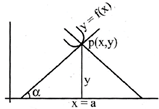
Let us consider a curve \[y=f(x)\] & take a point P\[(x,y)\] on it. We draw the tangent to the curve at \[P(x,y)\]which makes an angle \[\alpha \] with positive direction of x-axis. Then, \[{{\left. \frac{dy}{dx} \right|}_{\,\,at\,\,P(x,y)\,=\,tan\,\,\alpha \,=\,m(say)}}\] It is said to be gradient or slope of the tangent to the curve \[y=f(x)\]at\[p(x,y)\].  
    • Equation of the tangent: The equation of the tangent to a curve \[y=f(x)\] at the given point \[P({{x}_{1}},{{y}_{1}})\] is written in point slope form of the equation of straight more...

                                                                                                  Maxima and Minima of the Function  
    • Local maximum: A function \[y=f(x)\]is said to have local maximum value at a point\[x=a.\]
    If \[f(x)\le f(a)\]\[\forall x\in (a-h,a+h)\]and \[h>0\] i.e.\[f(a)\] is the greatest value of all values of \[f(x)\]in the interval\[(a-h,a+h)\] The point\[x=a\]is said to be the point of local maximum of the function     ·                    
    • Local minimum: A function\[y=f(x)\]is said to have a local minimum value at a point \[x=a.\] If
    \[f(x)\ge f(a)\]\[\forall x\in (a-h,a+h)\]for \[h>0\] i.e.\[f(a)\] is the smallest value of all the value of \[f(x)\] in the interval \[(a-h,a+h)\] The Point\[x=a\] is said to be the point of local minimum of the function\[f(x)\].   
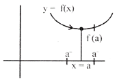
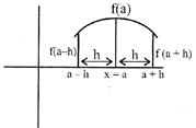
Note: The points at which the function attains either its maximum value or minimum value are said to be the extreme points of the function. Both the local maximum value and local minimum value of the function is said to be extreme value of the function. It is also said to be the relative maximum value and relative minimum value of the function respectively.  
    • Working rule to determine the point of local maxima and minima.
  • By 1st derivative method:
  • Procedure: (i) First of all find\[f'(x)\]and put\[f'(x)=0\] (ii) Solve it\[f'(x)=0\]and find the value of x. (iii) Let \[x=\alpha \]or\[\beta \]or\[\gamma \]etc. These points are said to be stationary points or critical points.     
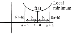
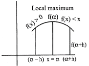
Let\[x=\alpha \]at any point (a) If \[f'(x)\] changes sign from positive to negative as x increase through a then\[x=\alpha \]is point of maximum. (b) If \[f'(x)\] changes sign from negative to positive as x increase through\[\alpha \]. Then\[x=\alpha \]is said to be the point of the minimum. 
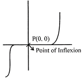
(c) If \[f'(x)\] does not change the sign as x increases through \[\alpha ,\] then\[x=\alpha \] is neither the point of maximum nor the point of minimum. Hence it is said to be the point of inflexion.   ·               
    • By Second Derivative Test:
    (i)  First of all find\[f'(x)\] & \[f''(x)\]of the given function\[y=f(x).\] (ii) Then put \[f'(x)=0\] to find the value of x. Let\[x=\alpha ,\beta \]and\[\gamma \] (a) If \[f''(x)<0,\]at\[x=\alpha ,\] then \[\alpha \] is said to be the point of local maximum and\[f(\alpha )\]is the maximum value of the function \[y=f(x).\] (b) If \[f''(x)>0\]at \[x=\alpha ,\] then \[\alpha \] is said to be the point of local minimum and\[f(\alpha )\]is the minimum value of the function \[y=f(x).\] (c) If\[f''(\alpha )=0\]then we cannot state anything about the function and we proceed the further derivatives and applying the same rule to check the maximum and minimum point of the function.  
  • Greatest and least value of the function in the more...

  •   Integral Calculus   Integration is the inverse process of differentiation i.e. the process of finding out the integral of the integrand function is called integration. e.g. If \[\frac{d}{dx}\{F(x)\}=f(x),\]then\[\int{f(x).dx=F(x)+C}\] Here function f(x) is said to be integrand and value of\[\int{f(x).dx=F(x)}\] is said to be integral value the function, \[c=\] Integration constant  
    • Some Basic Properties of Indefinite Integration
     
    Derivatives Integrals:
    1. \[\frac{d}{dx}({{x}^{n}})=n.{{x}^{n-1}}\] \[\int{{{x}^{n}}.dx=\frac{{{x}^{n}}+1}{n+1}+c}\] where \[c=\]integration constant.
    2. \[\frac{d}{dx}({{e}^{x}})={{e}^{x}}\] \[\int{{{e}^{x}}.dx={{e}^{x}}+c}\]
    3. \[\frac{d}{dx}\{\log (x)\}=\frac{1}{x}\] \[\int{\frac{1}{x}.dx=\log x+c}\]
    4. \[\frac{d}{dx}({{a}^{x}})={{a}^{x}}.\log a\] \[\int{{{a}^{x}}.dx=\frac{{{a}^{x}}}{\log a}+c}\]
    5. \[\frac{d}{dx}(\sin x)=\cos x\] \[\int{\cos x.dx=\sin x+c}\]
    6. \[\frac{d}{dx}(cosx)=-\sin x\] \[\int{\sin xdx=-\cos x+c}\]
    7. \[\frac{d}{dx}(tanx)={{\sec }^{2}}x\] \[\int{{{\sec }^{2}}xdx=\tan x+c}\]
    8. \[\frac{d}{dx}(cotx)=-\cos e{{c}^{2}}x\] \[\int{\cos e{{c}^{2}}xdx=-\cot x+c}\]
    9. \[\frac{d}{dx}(secx)=\sec x.\tan x\] \[\int{\sec x.\tan x.dx=\sec x+c}\]
    10. \[\frac{d}{dx}(cosecx)=-\cos ecx.\cot x\] \[\int{\cos ecx.cotx.dx=-\cos ec\,x+c}\]
    11. \[\frac{d}{dx}(ta{{n}^{-1}}x)=\frac{1}{1+{{x}^{2}}}\] \[\int{\frac{1}{1+{{x}^{2}}}.dx={{\tan }^{-1}}x+c}\]
    12. \[\frac{d}{dx}(si{{n}^{-1}}x)=\frac{1}{\sqrt{1-{{x}^{2}}}}\] \[\int{\frac{1}{\sqrt{1-{{x}^{2}}}}.dx={{\sin }^{-1}}x+c}\]
    13. \[\frac{d}{dx}(co{{s}^{-1}}x)=\frac{-1}{\sqrt{1-{{x}^{2}}}};\] \[\int{\frac{1}{\sqrt{1-{{x}^{2}}}}=-{{\cos }^{-1}}x+c}\]
    14. \[\frac{d}{dx}(ta{{n}^{-1}}x)=\frac{1}{1+{{x}^{2}}};\] \[\int{\frac{dx}{1+{{x}^{2}}}={{\tan }^{-1}}x+c}\]
    15. \[\frac{d}{dx}(-co{{t}^{-1}}x)=\frac{1}{1+{{x}^{2}}};\] \[\int{\frac{1}{1+{{x}^{2}}}dx=-{{\cot }^{-1}}x+c}\]
    16. \[\frac{d}{dx}(se{{c}^{-1}}x)=\frac{1}{x\sqrt{{{x}^{2}}-1}};\] \[\int{\frac{1}{x\sqrt{{{x}^{2}}-1}}.dx={{\sec }^{-1}}x+c}\]
    17. \[\frac{d}{dx}(-cose{{c}^{-1}}x)=\frac{1}{x\sqrt{{{x}^{2}}-1}};\] \[\int{\frac{dx}{x\sqrt{{{x}^{2}}-1}}=-\cos e{{c}^{-1}}x+c}\]
     
    • Method of Integration: The different methods of doing integration are as follows:
  • Method of transformation
  • Method of substitution
  • Method of Integration by parts
  •  
    • In method of transformation, we need to remember some basic trigonometry formulae that are being given below.
  • \[{{\sin }^{2}}x=\frac{1-\cos 2x}{2}\]
  • \[{{\cos }^{2}}x=\frac{1+\cos 2x}{2}\]
  • \[\sin 2x=2.\sin x\,\,\cos x\]
  • \[{{\sin }^{3}}x=\frac{3\sin x-\sin 3x}{4}\]
  • \[{{\cos }^{3}}x=\frac{3\cos x+\cos 3x}{4}\]
  • \[{{\tan }^{2}}x={{\sec }^{2}}x-1\]
  • \[{{\cot }^{2}}x=\cos e{{c}^{2}}x-1\]
  • \[2.\sin A.cosB=sin(A+B)+sin(A-B)\]
  • \[2.cosA.cosB=\cos (A+B)+\cos (A-B)\]
  • \[2.sinA.sinB=\cos (A-B)-\cos (A+B)\]
  •    
    • Integration by substitution: The given integral \[\int{f(x).dx}\] can be transformed into another form by changing the independent variable x to t.
    By substituting \[x=g(t).\] \[\because \]   Let us consider, \[I=\int{f(x).dx}\] Putting \[x=g(t)\]then\[dx=g'(t).dt\]\[\Rightarrow I=\int{f\{g(t)\}.g'(t).dt}\] This change of variable formula is one of the important tools available to us for integrating various functions.  
    • Some other Important Formulae of Integration
  • \[\int{\tan x.dx=\log more...

  •                                                                                  Differential Equations  
    • Definition: An equation involving independent variable, dependent variable and its derivatives is said to be differential equation.
    e.g. An equation of the form of \[\therefore \,\,\,\,\,y=f(x,y,p)\]is said to be differential equation, where\[p=\frac{dy}{dx}\]e.g. (1) \[y={{\left( \frac{dy}{dx} \right)}^{3}}+5\]              (2) \[{{x}^{2}}\frac{{{d}^{2}}y}{d{{x}^{2}}}+y\frac{dy}{dx}=5y+c\] etc.  
    • Order and Degree of differential Equation:
    The order of highest order derivative occurred in differential equation is said to be the order of the differential equation whereas power/exponent of the highest order derivative term in the different equation whereas power/exponent of the highest order derivative term in the differential equation is said to be the degree of the differential equation. e.g. (1) \[\frac{{{d}^{3}}y}{d{{x}^{3}}}+2{{\left( \frac{{{d}^{2}}y}{d{{x}^{2}}} \right)}^{2}}+6{{\left( \frac{dy}{dx} \right)}^{6}}+7y=0\] Here order of differential equation be 3 Degree of differential equation = 1 (2) \[{{\left[ 1+{{\left( \frac{dy}{dx} \right)}^{2}} \right]}^{\frac{3}{2}}}=\frac{{{d}^{3}}y}{d{{x}^{3}}}\] Order of this differential equation = 3 Degree of this differential equation = 2   Types of Differential Equation:
  • Ordinary Differential Equation: A differential equation involving single independent variable, is said to be an ordinary differential equation.
  • g. (1) \[\frac{dy}{dx}+6y=6{{x}^{2}}\] (2) \[\frac{{{d}^{2}}y}{d{{x}^{2}}}+2\frac{dy}{dx}+6y=0\]
  • Partial Differential Equation: A differential equation having two or more than two independent variables is said to be a partial differential equation.
  • If \[u=f(x,y,z),\] then its partial differential equation (P.D.E) will be \[\frac{{{\partial }^{2}}u}{\partial {{x}^{2}}}+\frac{{{\partial }^{2}}u}{\partial {{y}^{2}}}+\frac{{{\partial }^{2}}u}{\partial {{z}^{2}}}=0\]  
    • Methods for solving First Order, First Degree Differential equations:
    An equation of the form \[\frac{dy}{dx}=\frac{M}{N},\]where M and N be the functions of x and y or any constant value, is said to be the first order, first degree differential equation. This type of differential equation consists of following types of function
  • Separable function
  • Recudible seperable function
  • Homogeneous function and Non-Homogeneous function
  • Linear Differential equation
  • Recudible linear differential equation
  • Exact differential equation
  •   Solved Example
  • Find the general solution of differential equation \[\frac{dy}{dx}=(1+{{x}^{2}})(1+{{y}^{2}}).\]
  • Solution: \[\frac{dy}{dx}=(1+{{x}^{2}}).(1+{{y}^{2}})\] \[\Rightarrow \]   \[\frac{dy}{1+{{y}^{2}}}=(1+{{x}^{2}})dx\]              Integrating both sides, we get             \[{{\tan }^{-1}}y=x+\frac{{{x}^{3}}}{2}+c\] \[\Rightarrow \] \[y=\tan \left( \frac{2x+{{x}^{3}}+2c}{2} \right)\]  
    • Method for solving the Homogeneous differential equation
    Step 1: First of all arrange the given equation as \[\frac{dy}{dx}=\frac{\phi (x)}{f(x)},\] where \[\phi (x)\] and \[f(x)\] having same degree. Step2: Put\[y=\text{v}x\]and differentiate it on both sides to get \[\frac{dy}{dx}=\text{v}+x\frac{d\text{v}}{dx}\] Step 3: Then put these value in the given equation and further hence using variable seperable method, solution will be obtained in the form of v. Step 4: Then replace v by \[\frac{y}{x}\] & hence find the result.   Solved Example
  • Solve the differential equation \[y'=\frac{x+y}{x}.\]
  • Solution:\[y'=\frac{dx}{dx}=\frac{x+y}{x}.\]             (1) It is a homogeneous equation. Now, put \[y=\text{v}x\]                         (2) On differentiating both sides of equ (2), we get \[\frac{dy}{dx}=\text{v}+x\frac{d\text{v}}{dx}\] On replacing the value of \[\frac{dy}{dx}\] in equ (1), it becomes \[\text{v}+x\frac{d\text{v}}{dx}=\frac{x+\text{v}x}{x}=(1+\text{v})\] \[\Rightarrow \,\,\,x\frac{d.\text{v}}{dx}=1+\text{v}\,-\,\text{v=1}\]                     \[\Rightarrow \]            \[d\text{v}=\frac{dx}{x}\] On integrating both sides, we get \[\text{v}=\log x+\log c\] \[\frac{y}{x}=\log xc\](where log \[c=\] integration constant) \[y=x\log xc\] which is the required solution.  
    • Linear Differential Equation: An equation of the form of \[\frac{dy}{dx}+P.y=Q,\] more...

                                                                                                   Vector Algebra   ·                 
    • As we know that the some quantities have only magnitude and some have magnitude as well as direction, e.g. distance, force, work, current etc.
    On this basis, all physical quantities are divided into two groups: (i)  Scalar quantities. (ii) Vector quantities.  
    • Scalar quantity: A quantity which has only magnitude and does not have direction is said to be scalar quantity. For example: distance, speed, work-done etc.
     
    • Vector quantity: A quantity which has magnitude as well as direction and also obeys the addition law of triangle is said to be vector quantity. For example: Displacement, Force, Velocity etc.
     
    • Representation of vectors: A vector is symbolically represented by putting an arrow sign (\[\to \]) on a letter or group of letters representing directed line segment. For example, a vector drawn from a point 0 to point A. Point 0 is called the initial point and point A is called the end point. Symbolic notation for this vector is\[\left| \left. \overrightarrow{OA} \right| \right.\] .
     
    • Modulus (or magnitude) of a vector: The positive real number which is the measure of the length of the vector, is called the modulus, absolute value or length or magnitude or normal of the vector. For example, the magnitude of \[\vec{a}=2\hat{i}+3\hat{j}+5\hat{k}\]is given by, \[\left| \,\left. \vec{a}\, \right| \right.=\sqrt{{{(2)}^{2}}+{{(3)}^{2}}+{{(5)}^{2}}}\]\[=\sqrt{4+9+25}=\sqrt{38}\]
    where \[\hat{i}\],\[\hat{j}\] and \[\hat{k}\]are said to be the unit vectors.  
    • Position vector: The vector which gives the position of a point, relative to a fixed point (the origin) is called position vector.
    If \[P(x,y,z)\] be any point in space then position vector \[\overrightarrow{OP}=x\vec{i}+y\vec{j}+z\vec{k}\] \[\therefore \,\,|\,\,\overrightarrow{OP}\,\,|\]\[=\sqrt{{{x}^{2}}+{{y}^{2}}+{{z}^{2}}}\]  
    • Type of vectors:
  • Equal Vectors: Two vectors \[\vec{a}\] and \[\vec{b}\] are said to be equal, if they have the same magnitude and direction regardless of the positions of their initial points. They can be written as \[\vec{a}=\vec{b}\].
  •  
  • Negative of a Vector: A vector whose magnitude is the same as that of a given vector (say,\[\overrightarrow{PQ}\]), but direction is opposite to that of it, is called negative of the given vector. For example, vector \[\overrightarrow{QP}\] is negative of the vector \[\overrightarrow{PQ}\] i.e., \[\overrightarrow{QP}=-\overrightarrow{PQ}\]
  •  
  • Like and Unlike Vectors: Two vectors are said to be like vectors, if they have same direction. Similarly, two vectors are called unlike vectors, if they have opposite direction from each other.
  •  
  • Zero Vector: The vector whose initial and terminal points coincide, is called a zero vector or null vector. It is denoted as \[\vec{0}\]. Zero vector cannot be assigned a definite direction as it has zero magnitude. It is also said to have any direction. The vectors \[\overrightarrow{PP}\], \[\overrightarrow{QQ}\] represent the zero vector
  •  
  • Unit Vector: The vector whose magnitude is 1 unit or unity is known as unit vector. The unit vector more...

  •                                                                                Three Dimensional Geometry ·                
    • Direction cosines: Let P(a, b, c) be any point. We join P to origin O. Let the line OP makes an angle \[\alpha ,\beta ,\gamma \] with positive direction of x-axis, y-axis and z-axis respectively. Then \[\cos \alpha ,\cos \beta \] and \[\cos \gamma \] are called the direction cosine of the directed line OP. If the angle is measured in clockwise direction then the direction angles are replaced by their supplements i.e. \[\pi -\alpha ,\]\[\pi -\beta ,\]and\[\pi -\gamma \] respectively. It is generally denoted by \[\ell \], m and n respectively i.e. \[\ell =\cos \alpha ,\]\[m=\cos \beta \]and \[n-\cos \gamma \]
    \[\Rightarrow \] \[{{\ell }^{2}}+{{m}^{2}}+{{n}^{2}}=1\]  
    • Direction Ratio: The three number a, b, c proportional to the direction cosines \[\ell \]m, n of a vector are known as the direction ratio of the vector.
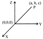
        Consider P(a, b, c) be any point in the space at length r from the origin to the axis. Here a, b and c are said to be direction ratios. \[\therefore OP=\sqrt{{{a}^{2}}+{{b}^{2}}+{{c}^{2}}}\] (By distance formula) \[|r|=\sqrt{{{a}^{2}}+{{b}^{2}}+{{c}^{2}}}\] Note: Direction cosine is proportional to the direction ratio. Let a, b, c be d.r.,s of the line OP and its d.c.'s be \[\ell \],m and n respectively. Then \[\frac{\ell }{a}=\frac{m}{b}=\frac{n}{c}=K\] (say) Convesion from direction ratios (d.r.'s) to direction cosines (d.c.'s) \[\ell =\pm \frac{a}{\sqrt{{{a}^{2}}+{{b}^{2}}+{{c}^{2}}}}\] \[m=\pm \frac{b}{\sqrt{{{a}^{2}}+{{b}^{2}}+{{c}^{2}}}}\] and \[n=\pm \frac{c}{\sqrt{{{a}^{2}}+{{b}^{2}}+{{c}^{2}}}}\]  
    • Some salient features of d.r.'s and d.c.'s
    If \[\vec{r}=a\hat{i}+b\hat{j}+c\hat{k}\] Then a, b and c be the d.r.'s of r and d.c.'s of r is given by \[\ell =\frac{a}{\sqrt{{{a}^{2}}+{{b}^{2}}+{{c}^{2}}}}\],\[m=\frac{b}{\sqrt{{{a}^{2}}+{{b}^{2}}+{{c}^{2}}}}\]and \[n=\frac{c}{\sqrt{{{a}^{2}}+{{b}^{2}}+{{c}^{2}}}}\]  
    • The D.R. of the line joining two points \[P({{x}_{1}},{{y}_{1}},{{z}_{1}})\]and\[Q({{x}_{2}},{{y}_{2}},{{z}_{2}})\]are \[{{x}_{2}}-{{x}_{1}},{{y}_{2}}-{{y}_{1}}\]and \[{{z}_{2}}-{{z}_{1}}\]and its direction cosines (d.c.'s) be \[\frac{{{x}_{2}}-{{x}_{1}}}{|PQ|},\]\[\frac{{{y}_{2}}-{{y}_{1}}}{|PQ|}\] and \[\frac{{{z}_{2}}-{{z}_{1}}}{|PQ|}\]respectively.
    • Direction cosines of x-axis, y-axis and z-axis be written as (1, 0, 0) (0, 1, 0) and (0, 0, 1) respectively.
     
    • Angle between two vectors: If \[\theta \] be the angle between two vectors whose direction cosines are
    \[{{\ell }_{1}},{{m}_{1}},{{n}_{1}}\]and \[{{\ell }_{2}},{{m}_{2}},{{n}_{2}}\]then \[\cos \theta ={{\ell }_{1}}{{\ell }_{2}}+{{m}_{1}}{{m}_{2}}+{{n}_{1}}{{n}_{2}}\] and\[\sin \theta =\sqrt{{{({{m}_{2}}{{\ell }_{1}}-{{m}_{1}}{{\ell }_{2}})}^{2}}-{{({{m}_{1}}{{n}_{2}}-{{m}_{2}}{{n}_{1}})}^{2}}+{{({{\ell }_{2}}{{n}_{1}}-{{\ell }_{1}}{{n}_{2}})}^{2}}}\]  
    • If\[{{\ell }_{1}}{{\ell }_{2}}+{{m}_{1}}{{m}_{2}}+{{n}_{1}}{{n}_{2}}=0\], then both vectors will be orthogonal.
     
    • If\[\frac{{{\ell }_{1}}}{{{\ell }_{2}}}=\frac{{{m}_{1}}}{{{m}_{2}}}=\frac{{{n}_{1}}}{{{n}_{2}}}\], then both vectors are parallel.
     
    • Angle in the terms of direction ratios (d.r.'s).
      If \[\vec{a}={{a}_{1}}\vec{i}+{{b}_{1}}\vec{j}+{{c}_{1}}\vec{k}\] and\[\vec{b}+{{a}_{2}}\vec{i}+{{b}_{2}}\vec{j}+{{c}_{2}}\vec{k}\]be the two vectors, then their direction ratios be \[{{a}_{1}},{{b}_{1}},{{c}_{1}}\] and \[{{a}_{2}},{{b}_{2}},{{c}_{2}}\] respectively. Let \[\theta \] is the .angle between these two vectors. Then \[\cos \theta =\]\[\frac{{{a}_{1}}{{a}_{2}}+{{b}_{1}}{{b}_{2}}+{{c}_{1}}{{c}_{2}}}{\sqrt{a_{1}^{2}+b_{1}^{2}+c_{1}^{2}}.\sqrt{a_{2}^{2}+b_{2}^{2}+c_{2}^{2}}}.\]  
    • If two vectors are orthogonal, then \[{{a}_{1}}.{{a}_{2}}+{{b}_{1}}.{{b}_{2}}+{{c}_{1}}.{{c}_{2}}=0\]
     
    • If two vectors are parallel, then \[\frac{{{a}_{1}}}{{{a}_{2}}}=\frac{{{b}_{1}}}{{{b}_{2}}}=\frac{{{c}_{1}}}{{{c}_{2}}}\]
     
    • Projection of the joining of the two points on a line: If \[P({{x}_{1}},{{y}_{1}},{{z}_{1}})\] and \[Q({{x}_{2}},{{y}_{2}},{{z}_{2}})\] are two points the length of the projection of PQ on a line whose more...

                                                                                     Probability    
    • Conditional Probability: The probability of event A is called the conditional probability of A given that event B has already occurred. It is written as \[P(A|B)\]or \[P\left( \frac{A}{B} \right)\].Mathematically it is given by the formula \[P(A|B)=\frac{P(A\bigcap B)}{P(B)}\]
    Event A is independent of B if the conditional probability of A given B is the same as the unconditional probability as A,i.e, they are independent if \[P(A|B)=P(A)\] 'Gender gap' in politics is a well-known example of conditional probability and independence in the real life. Suppose candidate A receive 55% of the entire vote and the only 45% of the female vote. Let \[P(R)=\] Probability that a random person voted for A But \[P\left( \frac{W}{R} \right)=\] Probability of a random women voted for A \[\therefore P(R)=0.55\]and \[P\left( \frac{W}{R} \right)=0.45\] Then \[P\left( \frac{W}{R} \right)\] is said to be the conditional probability of W given R.
    • If \[P(R)\ne P\left( \frac{W}{R} \right)\] then there exists a gender gap in politics. On the other hand. If \[P(A)=P\left( \frac{A}{W} \right),\] then there is no gender gap. i.e. the probability that a person voted for A is independent of the gender gap.
     
    • Independent Events: Let A and B be the two events. If\[P(A\bigcap B)=P(A).\,P(B)\], then A and B are said to be the independent events.
     
    • Mutually Exclusive Events: The events are said to be mutually exclusive, if the sets are disjoints i.e. \[P(A\bigcap B)=0\]i.e. \[A\bigcap B=\phi \]
    In such cases, \[P(A\bigcup B)=P(A)+P(B)\]  
    • Disjoint events/sets: Two sets or events are said to be disjoint if they have no element in common.
     
    • Properties of Conditional probability
  • If A and B be the events of a sample space Sand F is an event of S, then
  • \[P(S|F)=P(F|F)=1\]
  • If A and B are any two events of sample space S and F is an event of S such that \[P(F)\ne 0,\] then
  •             \[P[(A\bigcap B)|F]=P(A|F)+P(B|F)-P[A\bigcap B)|F]\] If A and B are disjoint events, then \[P[(A\bigcap B)|F]=P(A|F)+P(B|F)\]
  • \[P(A'|B)=1-P(A|B)\]
  •  
    • Law of Total Probability: Suppose S is a sample space and the subsets be \[{{A}_{1}},{{A}_{2}},{{A}_{3}},...{{A}_{k}},\] then any other event E is union of all the subsets. When \[E\cap {{A}_{k}}\] are disjoint, then
    \[P(E)=P(E\cap {{A}_{1}})+P(E\cap {{A}_{2}})+P(E\cap {{A}_{k}})\] Using the conditional theorem of probability, we have \[P(E\cap {{A}_{k}})=P({{A}_{k}}\cap E)=P({{A}_{k}}).P\left( \frac{E}{{{A}_{k}}} \right)\]  
    • Theorem of Total Probability: Let \[\{{{A}_{1}},{{A}_{2}},...{{A}_{n}}\}\] be a partition of sample space S and each of the event has non-zero probability. Let E be any event associated with S, then
    \[P(E)=P({{A}_{1}}).P\left( \frac{E}{{{A}_{1}}} \right)+P({{A}_{2}}).P\left( \frac{E}{{{A}_{2}}} \right)+...+P({{A}_{n}}).P\left( \frac{E}{{{A}_{n}}} \right)\] \[=\sum\limits_{i=1}^{n}{n}({{A}_{i}})P\left( \frac{E}{{{A}_{i}}} \right)\] This is known as theorem of total probability.  
    • Bayes' Theorem: Suppose the events \[{{A}_{1}},{{A}_{2}},...{{A}_{n}}\] form the partitions of the sample space S, i.e., \[{{A}_{1}},{{A}_{2}},...{{A}_{n}}\] are pairwise disjoint and \[{{A}_{1}}\cup {{A}_{2}}\cup ...\cup {{A}_{n}}=S\] and E is any event. Then
    \[P\left( \frac{{{A}_{i}}}{E} \right)=\frac{P({{A}_{i}}).P\left( \frac{E}{{{A}_{i}}} \right)}{P({{A}_{1}}).P\left( more...

    The technique of in-vitro fertilization and in-vitro development followed by the embryo-transfer in the uterus of the normal female to start the development and finally leading to normal birth, is called test tube baby. History : First attempt to produce a test tube baby was made by a Italian scientist, Dr. Petrucci (1959 A.D.). Although, this human embryo survived for only 29 days, but his experiment opened a new filed of biological science. The first test tube baby was born to Lesley and Gilbert Brown on July 25, 1978, in Oldham, England. Mrs. Brown had obstructed Fallopian tubes. Dr.Patiricke Steptoe and Dr. Robert Edward both from England experimented on Mrs. Brown successfully. the world's first test tube baby (a baby girl) was named as Louise Joy Brown. Later, test tube babies were also born in Australia, United States and some other countries. India's first test tube baby was born on 3rd October, 1978 in Kolkata. Her name was Kanupriya Aggarwal and was created by Dr. Subash Mukherjee. Procedure : It involves the following steps : (1) Removal of unfertilized ovum from reproductive tract of a female. (2) Ovum is kept under aseptic conditions. (3) Fusion of sperm and ovum in a culture medium, outside the female body, to form the zygote. (4) Zygote is stimulated to develop in vitro upto 32-celled stage. (5) Developing embryo is implanted on the endometrium of the uterus at 32-celled stage. So the pregnancy in the woman starts and further development of the child continues in the womb till it is born. Such a baby called a test tube baby. Significance (1) It is boon to infertile mothers. (2) It can be used for men with Oligospermia (low sperm count). (3) Old superior cows can donate oocytes. Embryos can be frozen and preserved in an embryo tank for 10 years for future use. In very rare cases, a surrogate mother may have to be used to bring up in vitro fertilized ovum to maturity. Though biological realization of a test baby is a remarkable achievement, it has raised several ethical and legal problems like the right over the child.

    Population Trends in the World The distribution of human population is not uniform throughout the world. Only about one third of the total land area is inhabited. Of the inhabited areas, some are thickly populated, others sparsely. This depends upon the availability of the requirements of life. About 56% of the total world population resides in Asia alone. Bangladesh is the most thickly populated country, and Australia, the most thinly populated. Annual Birth, Death and Growth Rates for Human Population in 1973
    S. No Region Population (Millions) Average Annual Birth Rate per 1,000 Individuals Average Annual Death Rate per 1,000 Individuals Annual Growth Rate Percent  
    (1) World 3860 33 13 2.0
    (2) Developed Countries 1120 more...
    Population : India’s population according to the provisional totals of Census of India 2001 at the 00.00 hours of Ist March 2001 is 1,027,015,247, out of which the population of Madhya Pradesh is 60,385,118, state thus contributing 5.87% share to India’s total population. Madhya Pradesh is the 7th largest state population-wise whereas it is 2nd in terms of its geographical spread and contributes 9.38% to the country’s total area of 3,287,263 sq.km.   Population 1901 to 2001 in Madhya Pradesh
    Year Population Year Population
    1901 12,679,214 1961 23,217,910
    1911 14,249,382 1971 30,016,625
    1921 13,906,774 1981 38,168,507
    1931 more...


    You need to login to perform this action.
    You will be redirected in 3 sec spinner