7th Class Computers Science Microsoft Excel Working With Microsoft Excel 2013

Working With Microsoft Excel 2013

 

Introduction

Microsoft Excel 2013 is a spreadsheet program that is used to manage, analyse and present data. Spreadsheet is an application software used for calculation based applications. In this application software, a user can edit and modify data and also calculates average, sum, difference, etc. A Spreadsheet contains rows and columns which forms many cells. There are 1, 048, 576 rows and 16, 384 columns in MS-Excel 2013. The Microsoft Excel opens with name, book 1, by default book 1 contain one sheet that can be renamed and additional worksheet can also be added in a work book 1. In the previous class, you have already read about some basic features of MS-Excel. In this chapter, we ?will study about the working with Microsoft Excel application software.

 

Entering Data in a Cell

Every cell in a worksheet has its own address. The data in a cell is entered by selecting a cell and pressing F2 key or double clicking the selected cell. Press enter or tab key to move to the next cell. Press Alt + Enter key on the keyboard to apply a line break. For over writing data in a cell, press Enter key after writing new data in a cell.

 

Moving the Content in a Worksheet

Moving the content from a selected range of cells into another location, move the contents to the new location. The cells must be selected using mouse or keyboard. You can use cut, copy and paste command to move or copy cells or their contents. To cut the selected range, right click the mouse and click on cut option from the drop down menu. Move the cursor at the corner of the first cell in which the item is to be moved. Now, click paste in the mouse right click drop down menu. Entire contents from the old location is moved into the new range of cells without leaving the old information. Whenever you copy or move a cell in Excel, it copies or moves the cell including formulas and their requesting values, cell formats and comments.

 

Deleting Data

You can delete the entire content of a cell if the data is no longer needed. Deleting data does not remove any formatting applied to the new data.

 

To delete data:

 

v  Select the cell that contain the data you want to delete, and then press the delete key.  

 

Filling a Range

The smallest area in which data is entered is the cell of a worksheet. Series of numbers can be inserted in a range of cells by clicking, (Editing  Fill  Series command) or dragging the fill handle.

 

 

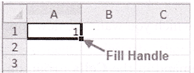
Fill Handle

Fill Handle in a cell is appeared after clicking in the cell. The lower right corner of a cell has i handle which appears as a solid square and when cursor is placed at the bottom right corner of the cell, a plus sign appears. The plus sign is dragged to fill range of cells in a worksheet.

 

 

Inserting Text Series Using Fill Handle

To insert text series in worksheet, such as inserting name of days starting from Sunday '"1 Saturday, first insert Sunday in a cell from where series is to be entered, now, drag the mouse to insert series of name of days.

 

Entering Date and Time in a Cell

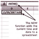
The NOW function, one of Excel date and time functions, is used to add the current date and time to a spreadsheet.                          

 

The syntax for the NOW function is: = NOW ( )

 

 

Note: The NOW function has no arguments. It obtains its formation on the current date and time by reading the Computer's serial date.

 

As a result, the function continually updates itself every time worksheet is recalculated.

 

Normally, worksheets recalculate each time they are opened so every day when the worksheet is opened, the date will change unless automatic recalculation is turned off. 

 

The following are the steps to insert date and time format in a cell of a worksheet:

 

• Click on the cell in which the date and time is to be inserted.
• Click on the Formulas
• Choose Date & Time from the ribbon to open the function drop down list.
• Click on NOW in the list to bring up the function's dialog box.
• Click
• The current date and time will appear in the cell.
• When you click on the cell, the complete function = NOW ( ) appears in the formula bar above the worksheet.
• If you want the cell to show only the current date or time, change the cell's format to show either date or time only.

 

 

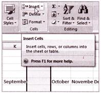
Inserting Rows and Columns in a Worksheet

 

To insert rows:

 

• Select the row above which you want the new row to appear.
• Click the Insert command in the Cells group on the Home The row will appear.
• The new row always appears above the selected row.

 

 

 

• Make sure that you have selected the entire row below where you want the new- row to appear and not just the cell. If you select just the cell and then click Insert, only a new cell will appear.

 

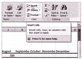
To insert columns:

 

• Select the column to the right where you want the column to appear.
• Click the Insert command in the Cells group on the Home The column will appear.
• The new column always appears to the left of the selected column. For example, if you want to insert a column between September and October, select the October column, then click the Insert command.

 

 

• Make sure that you have selected the entire column to the right of where you want the new column to appear and not just the cell. If you select just the cell and then click Insert, only a new cell will appear.

 

Types of Data Entered in a Spreadsheet

Data in a cell of a spreadsheet can be entered in the form of numbers, texts, formulas and special characters. The text entry in a cell of a Spreadsheet is also defined as the label. There are three types of data that can be entered in a spreadsheet.

 

Text (Label)

The text or label entry in a spreadsheet is defined as the entry of alphabets. It can contain letters, numbers and special characters like @, !, or &. By default, text data is left aligned in a cell.

 

Numbers

Numbers are entered in a spreadsheet for calculations or as raw data. Negative numbers -n a spreadsheet is entered with (-) sign. Parentheses can also be used for entering data. By default, numbers are right aligned in a cell.

 

Formulas

Formulas are entered in a spreadsheet to describe the relationship between cells. A forrmula may contain + (plus), - (minus), * (multiplication) or (division). In Microsoft Excel formula starts with an equal sign (=). The formula to calculate the sum of two numbers from two cells, A 10 and B10 will be =A10+B10. The equal sign indicates a forrmula and without equal sign, it is treated as a simple text only. Similarly, in the case of subtraction, the formula is inserted with the minus sign with the address, such as, for the subtraction of the value in cell A 15 from the value of A, the formula will be =A5-A15).

 

Chart in MS-Excel

A chart is a tool you can use in Excel to communicate your data graphically. Charts allow your audience to see the meaning behind the numbers in the spreadsheet more easily, and to make visual comparisons and trends much easier.

 

Types of charts in MS-Excel

There are many different types of charts available in MS-Excel some of them are discussed below:

 

 

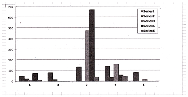
Column Chart

The column chart is used to compare values among one or more series of data points. In this chart, the vertical axis (y-axis) always displays numeric values and the horizontal axis (x-axis) displays time or other categories.

 

 

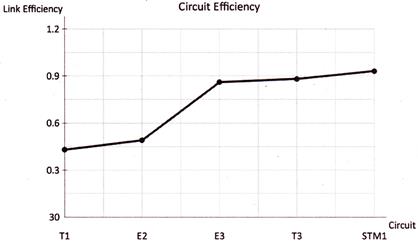
Line Chart

The line chart mainly displays trends over time. In this chart the x-axis displays time or other category and y-axis displays numerical values.

 

 

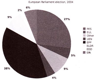
Pie Chart                                                     

A pie chart can display only one series of data. It displays the contribution of each value to the total.                                                                        

 

 

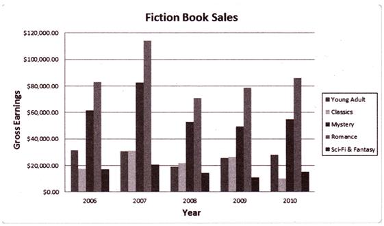
Bar Chart

The bar chart is just like a column chart but it can display and compare a large number : series better than .the column chart.

 

 

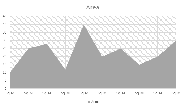
Area Chart

Area chart is just like the line chart but the difference is that the area below the plot -:ne is solid. It highlights differences between many sets of data over a period of time.

 

 

Scatter Chart

The scatter chart is also known as x, y chart. This chart compares the pairs of values.

 

 

Some of the other chart types used in MS-Excel are: stock, surface, doughnut, Bubble and Radar. But these charts are used very rarely by an average user.

 

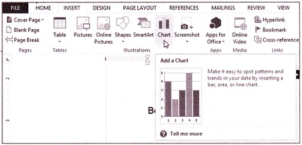
Creating a Chart

When you insert a chart in Excel, it appears in the selected worksheet with the source data by default.

 

To create a chart:

 

• Select the cells you want to create chart for including the column titles and row labels.
• Click the Insert tab, under Chart group.
• Select one of the Chart options. In this example, we are using the Column chart.
• Select a type of chart from the list that appears. In this example we are using 2-D clustered column chart that appears as shown below: