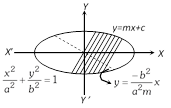
 The equation of the diameter bisecting the chords \[(y=mx+c)\] of slope \[m\] of the ellipse \[\frac{{{x}^{2}}}{{{a}^{2}}}+\frac{{{y}^{2}}}{{{b}^{2}}}=1\] is \[y=-\frac{{{b}^{2}}}{{{a}^{2}}m}x,\] which is passing through \[(0,\text{ }0)\].
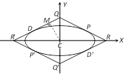
Conjugate diameter : Two diameters of an ellipse are said to be conjugate diameter if each bisects all chords parallel to the other. The coordinates of the four extremities of two conjugate diameters are
The equation of the diameter bisecting the chords \[(y=mx+c)\] of slope \[m\] of the ellipse \[\frac{{{x}^{2}}}{{{a}^{2}}}+\frac{{{y}^{2}}}{{{b}^{2}}}=1\] is \[y=-\frac{{{b}^{2}}}{{{a}^{2}}m}x,\] which is passing through \[(0,\text{ }0)\].
Conjugate diameter : Two diameters of an ellipse are said to be conjugate diameter if each bisects all chords parallel to the other. The coordinates of the four extremities of two conjugate diameters are
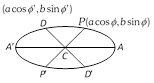
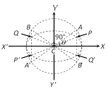 \[P(a\cos \varphi ,b\sin \varphi )\,;\,{P}'(-a\cos \varphi ,-b\sin \varphi )\]
\[Q(-a\sin \varphi ,\,b\cos \varphi );\,{Q}'(a\sin \varphi ,\,-b\cos \varphi )\]
If \[y={{m}_{1}}x\]and \[y={{m}_{2}}x\] be two conjugate diameters of an ellipse, then \[{{m}_{1}}{{m}_{2}}=\frac{-{{b}^{2}}}{{{a}^{2}}}\].
(1) Properties of diameters : (i) The tangent at the extremity of any diameter is parallel to the chords it bisects or parallel to the conjugate diameter.
(ii) The tangent at the ends of any chord meet on the diameter which bisects the chord.
(2) Properties of conjugate diameters : (i) The eccentric angles of the ends of a pair of conjugate diameters of an ellipse differ by a right angle, i.e., \[\varphi -{\varphi }'=\frac{\pi }{2}\].
\[P(a\cos \varphi ,b\sin \varphi )\,;\,{P}'(-a\cos \varphi ,-b\sin \varphi )\]
\[Q(-a\sin \varphi ,\,b\cos \varphi );\,{Q}'(a\sin \varphi ,\,-b\cos \varphi )\]
If \[y={{m}_{1}}x\]and \[y={{m}_{2}}x\] be two conjugate diameters of an ellipse, then \[{{m}_{1}}{{m}_{2}}=\frac{-{{b}^{2}}}{{{a}^{2}}}\].
(1) Properties of diameters : (i) The tangent at the extremity of any diameter is parallel to the chords it bisects or parallel to the conjugate diameter.
(ii) The tangent at the ends of any chord meet on the diameter which bisects the chord.
(2) Properties of conjugate diameters : (i) The eccentric angles of the ends of a pair of conjugate diameters of an ellipse differ by a right angle, i.e., \[\varphi -{\varphi }'=\frac{\pi }{2}\].
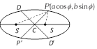
 (ii) The sum of the squares of any two conjugate semi-diameters of an ellipse is constant and equal to the sum of the squares of the semi axes of the ellipse i.e.,\[C{{P}^{2}}+C{{D}^{2}}={{a}^{2}}+{{b}^{2}}\].
(iii) The product of the focal distances of a point on an ellipse is equal to the square of the semi-diameter which is conjugate to the diameter through the point i.e., \[SP.{S}'P=C{{D}^{2}}\].
(ii) The sum of the squares of any two conjugate semi-diameters of an ellipse is constant and equal to the sum of the squares of the semi axes of the ellipse i.e.,\[C{{P}^{2}}+C{{D}^{2}}={{a}^{2}}+{{b}^{2}}\].
(iii) The product of the focal distances of a point on an ellipse is equal to the square of the semi-diameter which is conjugate to the diameter through the point i.e., \[SP.{S}'P=C{{D}^{2}}\].
 (iv) The tangents at the extremities of a pair of conjugate diameters form a parallelogram whose area is constant and equal to product of the axes. i.e., Area of parallelogram \[=(2a)(2b)\] = Area of rectangle contained under major and minor axes.
 (v) The polar of any point with respect to ellipse is parallel to the diameter to the one on which the point lies. Hence obtain the equation of the chord whose mid point is \[({{x}_{1,}}{{y}_{1}})\], i.e. chord is \[T={{S}_{1}}\].
(3) Equi-conjugate diameters: Two conjugate diameters are called equi-conjugate, if their lengths are equal i.e., \[{{(CP)}^{2}}={{(CD)}^{2}}\].
\[\therefore \] \[(CP)=(CD)=\sqrt{\frac{({{a}^{2}}+{{b}^{2}})}{2}}\] for equi-conjugate diameters.
(v) The polar of any point with respect to ellipse is parallel to the diameter to the one on which the point lies. Hence obtain the equation of the chord whose mid point is \[({{x}_{1,}}{{y}_{1}})\], i.e. chord is \[T={{S}_{1}}\].
(3) Equi-conjugate diameters: Two conjugate diameters are called equi-conjugate, if their lengths are equal i.e., \[{{(CP)}^{2}}={{(CD)}^{2}}\].
\[\therefore \] \[(CP)=(CD)=\sqrt{\frac{({{a}^{2}}+{{b}^{2}})}{2}}\] for equi-conjugate diameters. 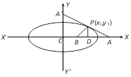 \[DA=CA-CD=\frac{{{a}^{2}}}{{{x}_{1}}}-{{x}_{1}}\].
Length of sub-normal at \[P({{x}_{1,}}{{y}_{1}})\]to the ellipse \[\frac{{{x}^{2}}}{{{a}^{2}}}+\frac{{{y}^{2}}}{{{b}^{2}}}=1\] is \[BD=CD-CB={{x}_{1}}-\left( {{x}_{1}}-\frac{{{b}^{2}}}{{{a}^{2}}}{{x}_{1}} \right)\]\[=\frac{{{b}^{2}}}{{{a}^{2}}}{{x}_{1}}=(1-{{e}^{2}}){{x}_{1}}\].
\[DA=CA-CD=\frac{{{a}^{2}}}{{{x}_{1}}}-{{x}_{1}}\].
Length of sub-normal at \[P({{x}_{1,}}{{y}_{1}})\]to the ellipse \[\frac{{{x}^{2}}}{{{a}^{2}}}+\frac{{{y}^{2}}}{{{b}^{2}}}=1\] is \[BD=CD-CB={{x}_{1}}-\left( {{x}_{1}}-\frac{{{b}^{2}}}{{{a}^{2}}}{{x}_{1}} \right)\]\[=\frac{{{b}^{2}}}{{{a}^{2}}}{{x}_{1}}=(1-{{e}^{2}}){{x}_{1}}\]. 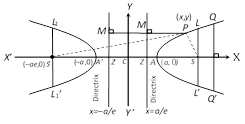
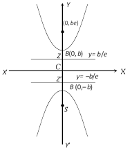 Difference between both hyperbolas will be clear from the following table :
| Hyperbola | \[\frac{{{x}^{\mathbf{2}}}}{{{a}^{\mathbf{2}}}}-\frac{{{y}^{\mathbf{2}}}}{{{b}^{\mathbf{2}}}}=\mathbf{1}\] | \[-\frac{{{x}^{\mathbf{2}}}}{{{a}^{\mathbf{2}}}}+\frac{{{y}^{\mathbf{2}}}}{{{b}^{\mathbf{2}}}}=\mathbf{1}\] or \[\frac{{{x}^{\mathbf{2}}}}{{{a}^{\mathbf{2}}}}-\frac{{{y}^{\mathbf{2}}}}{{{b}^{\mathbf{2}}}}=-\mathbf{1}\] |
| Imp. terms | ||
| Centre | \[(0,\,\,0)\] | \[(0,\,\,0)\] |
| Length of transverse axis | \[2a\] | \[2b\] |
| Length of conjugate axis | \[2b\] | \[2a\] |
| Foci | \[(\pm \,ae,\,0)\] | \[(0,\,\pm be)\] |
| Equation of directrices | \[x=\pm a/e\] | \[y=\pm b/e\] |
| more...
If the centre of hyperbola is \[(h,\,\,k)\] and axes are parallel to the co-ordinate axes, then its equation is \[\frac{{{(x-h)}^{2}}}{{{a}^{2}}}-\frac{{{(y-k)}^{2}}}{{{b}^{2}}}=1\].
Let \[\frac{{{x}^{2}}}{{{a}^{2}}}-\frac{{{y}^{2}}}{{{b}^{2}}}=1\] be the hyperbola, then equation of the auxiliary circle is \[{{x}^{2}}+{{y}^{2}}={{a}^{2}}\].
Let \[\angle QCN=\varphi \]. Here P and Q are the corresponding points on the hyperbola and the auxiliary circle \[(0\le \varphi <2\pi )\].
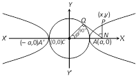
The equations \[x=a\sec \varphi \] and \[y=b\tan \varphi \] are known as the parametric equations of the hyperbola \[\frac{{{x}^{2}}}{{{a}^{2}}}-\frac{{{y}^{2}}}{{{b}^{2}}}=1\]. This \[(a\sec \varphi ,\,b\tan \varphi )\] lies on the hyperbola for all values of \[\varphi \].
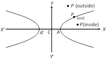
Let the hyperbola be \[\frac{{{x}^{2}}}{{{a}^{2}}}-\frac{{{y}^{2}}}{{{b}^{2}}}=1\].
Then \[P({{x}_{1}},\,{{y}_{1}})\] will lie inside, on or outside the hyperbola \[\frac{{{x}^{2}}}{{{a}^{2}}}-\frac{{{y}^{2}}}{{{b}^{2}}}=1\] according as \[\frac{x_{1}^{2}}{{{a}^{2}}}-\frac{y_{1}^{2}}{{{b}^{2}}}-1\] is positive, zero or negative.
The straight line \[y=mx+c\] will cut the hyperbola \[\frac{{{x}^{2}}}{{{a}^{2}}}-\frac{{{y}^{2}}}{{{b}^{2}}}=1\] in two points may be real, coincident or imaginary according as \[{{c}^{2}}>,\,=,\,<{{a}^{2}}{{m}^{2}}-{{b}^{2}}\].
Condition of tangency : If straight line \[y=mx+c\] touches the hyperbola \[\frac{{{x}^{2}}}{{{a}^{2}}}-\frac{{{y}^{2}}}{{{b}^{2}}}=1\], then \[{{c}^{2}}={{a}^{2}}{{m}^{2}}-{{b}^{2}}\].
Current Affairs CategoriesArchive
Trending Current Affairs


You need to login to perform this action. |

