 \[\omega -\] Angular speed
\[v-\] Frequency of rotation of coil
\[R-\]Resistance of coil
For uniform rotational motion with \[\omega ,\] the flux linked with coil at any time t
\[\varphi =NBA\cos \theta =NBA\cos \omega t\]
\[\phi ={{\phi }_{0}}\cos \,\omega t\] where \[{{\phi }_{0}}=NBA=\] maximum flux
(1) Induced emf in coil : Induced emf also changes in periodic manner that?s why this phenomenon called periodic EMI
\[e=-\frac{d\varphi }{dt}=NBA\omega \sin \omega \,t\]\[\Rightarrow \]\[e={{e}_{0}}\sin \,\omega t\] where \[{{e}_{0}}=emf\] amplitude or max. emf \[=NBA\omega ={{\varphi }_{0}}\omega \]
(2) Induced current : At any time t, \[i=\frac{e}{R}=\frac{{{e}_{0}}}{R}\sin \omega \,t={{i}_{0}}\sin \omega \,t\] where \[{{i}_{0}}=\] current amplitude or max. current \[{{i}_{0}}=\frac{{{e}_{0}}}{R}=\frac{NBA\omega }{R}=\frac{{{\varphi }_{0}}\omega }{R}\]
\[\omega -\] Angular speed
\[v-\] Frequency of rotation of coil
\[R-\]Resistance of coil
For uniform rotational motion with \[\omega ,\] the flux linked with coil at any time t
\[\varphi =NBA\cos \theta =NBA\cos \omega t\]
\[\phi ={{\phi }_{0}}\cos \,\omega t\] where \[{{\phi }_{0}}=NBA=\] maximum flux
(1) Induced emf in coil : Induced emf also changes in periodic manner that?s why this phenomenon called periodic EMI
\[e=-\frac{d\varphi }{dt}=NBA\omega \sin \omega \,t\]\[\Rightarrow \]\[e={{e}_{0}}\sin \,\omega t\] where \[{{e}_{0}}=emf\] amplitude or max. emf \[=NBA\omega ={{\varphi }_{0}}\omega \]
(2) Induced current : At any time t, \[i=\frac{e}{R}=\frac{{{e}_{0}}}{R}\sin \omega \,t={{i}_{0}}\sin \omega \,t\] where \[{{i}_{0}}=\] current amplitude or max. current \[{{i}_{0}}=\frac{{{e}_{0}}}{R}=\frac{NBA\omega }{R}=\frac{{{\varphi }_{0}}\omega }{R}\] 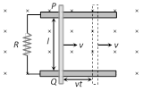 As shown in figure in time t distance travelled by conductor = vt
Area generated \[A=lvt\]. Flux linked with this area \[\phi =BA=Blvt\]. Hence induced emf \[|e|\,=\frac{d\varphi }{dt}=Bvl\]
(1) Induced current : \[i=\frac{e}{R}\]\[=\frac{Bvl}{R}\]
(2) Magnetic force : Conductor PQ experiences a magnetic force in opposite direction of it's motion and \[{{F}_{m}}=Bil=B\left( \frac{Bvl}{R} \right)\,l\]\[=\frac{{{B}^{2}}v{{l}^{2}}}{R}\]
(3) Power dissipated in moving the conductor : For uniform motion of rod PQ, the rate of doing mechanical work by external agent or mech. Power delivered by external source is given as \[{{P}_{mech}}={{P}_{ext}}=\frac{dW}{dt}={{F}_{ext}}.\,v=\frac{{{B}^{2}}v{{l}^{2}}}{R}\times v\]\[=\frac{{{B}^{2}}{{v}^{2}}{{l}^{2}}}{R}\]
(4) Electrical power : Also electrical power dissipated in resistance or rate of heat dissipation across resistance is given as \[{{P}_{thermal}}=\frac{H}{t}={{i}^{2}}R={{\left( \frac{Bvl}{R} \right)}^{2}}.R\];\[{{P}_{thermal}}=\frac{{{B}^{2}}{{v}^{2}}{{l}^{2}}}{R}\]
(It is clear that \[{{P}_{mech.}}={{P}_{thermal}}\] which is consistent with the principle of conservation of energy.)
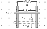
(5) Motion of conductor rod in a vertical plane : If conducting rod released from rest (at \[t=0\]) as shown in figure then with rise in it's speed (v), induces emf (e), induced current (i), magnetic force \[({{F}_{m}})\] increases but it's weight remains constant.
Rod will achieve a constant maximum (terminal) velocity \[{{v}_{T}}\] if \[{{F}_{m}}=mg\] So \[\frac{{{B}^{2}}v_{T}^{2}{{l}^{2}}}{R}=mg\] \[\Rightarrow \] \[{{v}_{T}}=\frac{mgR}{{{B}^{2}}{{l}^{2}}}\]
As shown in figure in time t distance travelled by conductor = vt
Area generated \[A=lvt\]. Flux linked with this area \[\phi =BA=Blvt\]. Hence induced emf \[|e|\,=\frac{d\varphi }{dt}=Bvl\]
(1) Induced current : \[i=\frac{e}{R}\]\[=\frac{Bvl}{R}\]
(2) Magnetic force : Conductor PQ experiences a magnetic force in opposite direction of it's motion and \[{{F}_{m}}=Bil=B\left( \frac{Bvl}{R} \right)\,l\]\[=\frac{{{B}^{2}}v{{l}^{2}}}{R}\]
(3) Power dissipated in moving the conductor : For uniform motion of rod PQ, the rate of doing mechanical work by external agent or mech. Power delivered by external source is given as \[{{P}_{mech}}={{P}_{ext}}=\frac{dW}{dt}={{F}_{ext}}.\,v=\frac{{{B}^{2}}v{{l}^{2}}}{R}\times v\]\[=\frac{{{B}^{2}}{{v}^{2}}{{l}^{2}}}{R}\]
(4) Electrical power : Also electrical power dissipated in resistance or rate of heat dissipation across resistance is given as \[{{P}_{thermal}}=\frac{H}{t}={{i}^{2}}R={{\left( \frac{Bvl}{R} \right)}^{2}}.R\];\[{{P}_{thermal}}=\frac{{{B}^{2}}{{v}^{2}}{{l}^{2}}}{R}\]
(It is clear that \[{{P}_{mech.}}={{P}_{thermal}}\] which is consistent with the principle of conservation of energy.)
(5) Motion of conductor rod in a vertical plane : If conducting rod released from rest (at \[t=0\]) as shown in figure then with rise in it's speed (v), induces emf (e), induced current (i), magnetic force \[({{F}_{m}})\] increases but it's weight remains constant.
Rod will achieve a constant maximum (terminal) velocity \[{{v}_{T}}\] if \[{{F}_{m}}=mg\] So \[\frac{{{B}^{2}}v_{T}^{2}{{l}^{2}}}{R}=mg\] \[\Rightarrow \] \[{{v}_{T}}=\frac{mgR}{{{B}^{2}}{{l}^{2}}}\]
 Special cases Motion of train and aeroplane in earth's magnetic field
 Induced emf across the axle of the wheels of the train and it is across the tips of the wing of the aeroplane is given by \[e={{B}_{v}}lv\] where \[l=\] length of the axle or distance between the tips of the wings of plane, \[{{B}_{v}}=\] vertical component of earth's magnetic field and v = speed of train or plane.
 | Lens | Focal length | For \[\mu =1.5\] |
|
Biconvex lens
|
\[f=\frac{R}{2(\mu -1)}\] | \[f=R\] |
|
Plano-convex lens
|
\[f=\frac{R}{(\mu -1)}\] | \[f=2R\] |
|
Biconcave
|
\[f=-\frac{R}{2(\mu -1)}\] | \[f=-R\] |
|
Plano-concave
|
\[f=\frac{-R}{(\mu -1)}\] | \[f=-2R\] |
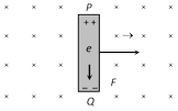 Conducting electrons experiences a magnetic force \[{{F}_{m}}=evB.\] So they move from P to Q within the rod. The end P of the rod becomes positively charged while end Q becomes negatively charged, hence an electric field is set up within the rod which opposes the further downward movement of electrons i.e. an equilibrium is reached and in equilibrium \[{{F}_{e}}={{F}_{m}}\] i.e. \[eE=evB\] or \[E=vB\Rightarrow \] Induced emf \[e=El=Bvl\] [\[E=\frac{V}{l}\]]
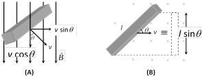
(2) If rod is moving by making an angle \[\theta \] with the direction of magnetic field or length. Induced emf \[e=Bvl\sin \theta \]
Conducting electrons experiences a magnetic force \[{{F}_{m}}=evB.\] So they move from P to Q within the rod. The end P of the rod becomes positively charged while end Q becomes negatively charged, hence an electric field is set up within the rod which opposes the further downward movement of electrons i.e. an equilibrium is reached and in equilibrium \[{{F}_{e}}={{F}_{m}}\] i.e. \[eE=evB\] or \[E=vB\Rightarrow \] Induced emf \[e=El=Bvl\] [\[E=\frac{V}{l}\]]
(2) If rod is moving by making an angle \[\theta \] with the direction of magnetic field or length. Induced emf \[e=Bvl\sin \theta \]
 (3) Motion of conducting rod on an inclined plane : When conductor start sliding from the top of an inclined plane as shown, it moves perpendicular to it?s length but at an angle \[(90-\theta )\]with the direction of magnetic field.
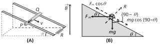 Hence induced emf across the ends of conductor \[e=Bv\sin (90-\theta )l=Bvl\cos \theta \]
So induced current \[i=\frac{Bvl\cos \theta }{R}\] (Directed from Q to P).
The forces acting on the bar are shown in following figure. The rod will move down with constant velocity only if
\[{{F}_{m}}\cos \theta =mg\cos (90-\theta )\]\[=mg\sin \theta \]\[\Rightarrow \]\[Bil\cos \theta =mg\sin \theta \]
\[B\left( \frac{B{{v}_{T}}l\cos \theta }{R} \right)\,l\cos \theta =mg\sin \theta \]\[\Rightarrow \]\[{{v}_{T}}=\frac{mgR\sin \,\theta }{{{B}^{2}}{{l}^{2}}{{\cos }^{2}}\theta }\]
Hence induced emf across the ends of conductor \[e=Bv\sin (90-\theta )l=Bvl\cos \theta \]
So induced current \[i=\frac{Bvl\cos \theta }{R}\] (Directed from Q to P).
The forces acting on the bar are shown in following figure. The rod will move down with constant velocity only if
\[{{F}_{m}}\cos \theta =mg\cos (90-\theta )\]\[=mg\sin \theta \]\[\Rightarrow \]\[Bil\cos \theta =mg\sin \theta \]
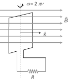
\[B\left( \frac{B{{v}_{T}}l\cos \theta }{R} \right)\,l\cos \theta =mg\sin \theta \]\[\Rightarrow \]\[{{v}_{T}}=\frac{mgR\sin \,\theta }{{{B}^{2}}{{l}^{2}}{{\cos }^{2}}\theta }\] 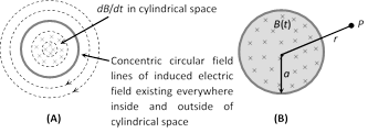 A uniform but time varying magnetic field B(t) exists in a circular region of radius 'a' and is directed into the plane of the paper as shown, the magnitude of the induced electric field \[({{E}_{in}})\] at point P lies at a distance r from the centre of the circular region is calculated as follows.
So \[\oint{{{{\vec{E}}}_{in}}d\vec{l}}=e=\frac{d\varphi }{dt}=A\frac{dB}{dt}\] i.e. \[E(2\pi r)=\pi {{a}^{2}}\frac{dB}{dt}\]
where \[r\ge a\] or \[E=\frac{{{a}^{2}}}{2r}\frac{dB}{dt}\]; \[{{E}_{\mathbf{in}}}\propto \frac{1}{r}\]
A uniform but time varying magnetic field B(t) exists in a circular region of radius 'a' and is directed into the plane of the paper as shown, the magnitude of the induced electric field \[({{E}_{in}})\] at point P lies at a distance r from the centre of the circular region is calculated as follows.
So \[\oint{{{{\vec{E}}}_{in}}d\vec{l}}=e=\frac{d\varphi }{dt}=A\frac{dB}{dt}\] i.e. \[E(2\pi r)=\pi {{a}^{2}}\frac{dB}{dt}\]
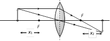
where \[r\ge a\] or \[E=\frac{{{a}^{2}}}{2r}\frac{dB}{dt}\]; \[{{E}_{\mathbf{in}}}\propto \frac{1}{r}\] 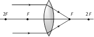 \[\to \] At F
\[\to \] Real
\[\to \] Inverted
\[\to \] Very small in size
Magnification \[m<<-1\]
(2) When object is placed between infinite and 2F (i.e. \[u>2f\])
Image
\[\to \] At F
\[\to \] Real
\[\to \] Inverted
\[\to \] Very small in size
Magnification \[m<<-1\]
(2) When object is placed between infinite and 2F (i.e. \[u>2f\])
Image
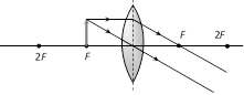
 \[\to \] Between F and 2F
\[\to \] Real
\[\to \] Inverted
\[\to \] Very small in size
Magnification \[m<-1\]
(3) When object is placed at 2F (i.e. \[u=2f\])
Image
\[\to \] Between F and 2F
\[\to \] Real
\[\to \] Inverted
\[\to \] Very small in size
Magnification \[m<-1\]
(3) When object is placed at 2F (i.e. \[u=2f\])
Image
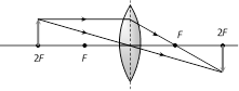 \[\to \] At 2F
\[\to \] Real
\[\to \] Inverted
\[\to \] Equal in size
Magnification \[m=-1\]
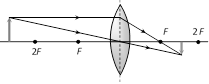
(4) When object is placed between F and 2F (i.e. \[f<u<2f\])
Image
\[\to \] At 2F
\[\to \] Real
\[\to \] Inverted
\[\to \] Equal in size
Magnification \[m=-1\]
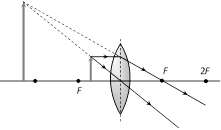
(4) When object is placed between F and 2F (i.e. \[f<u<2f\])
Image
 \[\to \] Beyond 2F
\[\to \] Real
\[\to \] Inverted
\[\to \] Large in size
\[\to \] Magnification \[m>-1\]
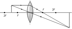
(5) When object is placed at F (i.e. \[u=f\] )
Image
\[\to \] Beyond 2F
\[\to \] Real
\[\to \] Inverted
\[\to \] Large in size
\[\to \] Magnification \[m>-1\]
(5) When object is placed at F (i.e. \[u=f\] )
Image
 \[\to \] At \[\infty \
] \[\to \] Real
\[\to \] Inverted
\[\to \] Very large in size
Magnification \[m>>-1\]
(6) When object is placed between F and optical center (i.e. \[u<f\])
Image
\[\to \] At \[\infty \
] \[\to \] Real
\[\to \] Inverted
\[\to \] Very large in size
Magnification \[m>>-1\]
(6) When object is placed between F and optical center (i.e. \[u<f\])
Image
 \[\to \] Same side as that of object
\[\to \] Virtual
\[\to \] Erect large in size
Magnification \[m>1\]
Concave lens : The image formed by a concave lens is always virtual, erect and diminished (like a convex mirror)
(1) When object is placed at \[\infty \]
Image
\[\to \] Same side as that of object
\[\to \] Virtual
\[\to \] Erect large in size
Magnification \[m>1\]
Concave lens : The image formed by a concave lens is always virtual, erect and diminished (like a convex mirror)
(1) When object is placed at \[\infty \]
Image
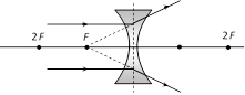 \[\to \] At F
\[\to \] Virtual
\[\to \] Erect
\[\to \] Point size
Magnification \[m<<+1\]
(2) When object is placed any where on the principal axis
Image
\[\to \] At F
\[\to \] Virtual
\[\to \] Erect
\[\to \] Point size
Magnification \[m<<+1\]
(2) When object is placed any where on the principal axis
Image
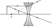 \[\to \] Between optical centre and focus
\[\to \] Virtual
\[\to \] Erect
\[\to \] Smaller in size
Magnification \[m<+1\]
\[\to \] Between optical centre and focus
\[\to \] Virtual
\[\to \] Erect
\[\to \] Smaller in size
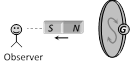
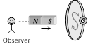
Magnification \[m<+1\] 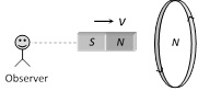 The various positions of relative motion between the magnet and the coil
| Position of magnet | 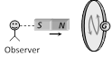 |
 |
 |
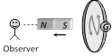 |
| Direction of induced current | Anticlockwise direction | Clockwise direction | Clockwise direction | Anticlockwise direction |
| Behaviour of face of the coil | As a north pole | As a more...
(1) Focal length (f) : Distance of second principle focus from optical centre is called focal length
\[{{f}_{\text{convex}}}\to \]positive, \[{{f}_{\text{concave}}}\to \]negative, \[{{f}_{\text{plane}}}\to \infty \]
(2) Aperture : Effective diameter of light transmitting area is called aperture. \[\text{Intensity of image }\propto {{\text{(Aperture)}}^{\text{2}}}\]
(3) Power of lens (P) : Means the ability of a lens to deviate the path of the rays passing through it. If the lens converges the rays parallel to the principal axis its power is positive and if it diverges the rays it is negative.
Power of lens\[P=\frac{1}{f(m)}=\frac{100}{f(cm)}\]; Unit of power is Diopter (D)
\[{{P}_{\text{convex}}}\to \text{positive,}\]\[{{P}_{\text{concave}}}\to \text{negative,}\]\[{{P}_{\text{plane}}}\to \text{zero}\].
Current Affairs CategoriesArchive
Trending Current Affairs


You need to login to perform this action. |

