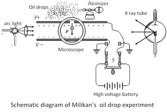
 where \[\eta =\] Coefficient of viscosity of air, \[{{v}_{1}}=\] Terminal velocity of drop when no electric field is applied between the plates, \[{{v}_{2}}=\] Terminal velocity of drop when electric field is applied between the plates.
V = Potential difference between the plates, d = Separation between plates, \[\rho =\] density of oil, \[\sigma =\]Density of air.
where \[\eta =\] Coefficient of viscosity of air, \[{{v}_{1}}=\] Terminal velocity of drop when no electric field is applied between the plates, \[{{v}_{2}}=\] Terminal velocity of drop when electric field is applied between the plates.
V = Potential difference between the plates, d = Separation between plates, \[\rho =\] density of oil, \[\sigma =\]Density of air. 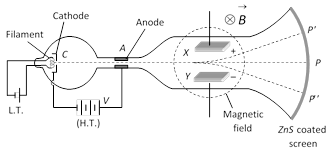 In this case; Electric force = Magnetic force
\[\Rightarrow \] eE = evB \[\Rightarrow \] \[v=\frac{E}{B};\] v = velocity of electron
(5) As electron beam accelerated from cathode to anode its loss in potential energy appears as gain in the K.E. at the anode. If suppose V is the potential difference between cathode and anode then, loss in potential energy = eV
And gain in kinetic energy at anode will be K.E. \[=\frac{1}{2}m{{v}^{2}}\] i.e.
\[eV=\frac{1}{2}m{{v}^{2}}\]\[\Rightarrow \]\[\frac{e}{m}=\frac{{{v}^{2}}}{2V}\]\[\Rightarrow \]\[\frac{e}{m}=\frac{{{E}^{2}}}{2V{{B}^{2}}}\]
Thomson found, \[\frac{e}{m}=1.77\times {{10}^{11}}C/kg.\]
If one includes the relativistic variation of mass with speed \[(m={{m}_{0}}/\sqrt{1-{{v}^{2}}/{{c}^{2}}})\], then specific charge of an electron decreases with the increase in its velocity.
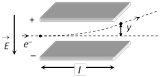
(6) The deflection of an electron in a purely electric field is given by \[y=\frac{1}{2}\left( \frac{eE}{m} \right).\frac{{{l}^{2}}}{{{v}^{2}}}\]; where l = Length of each plate, y = deflection of electron in the field region, v = speed of the electron.
In this case; Electric force = Magnetic force
\[\Rightarrow \] eE = evB \[\Rightarrow \] \[v=\frac{E}{B};\] v = velocity of electron
(5) As electron beam accelerated from cathode to anode its loss in potential energy appears as gain in the K.E. at the anode. If suppose V is the potential difference between cathode and anode then, loss in potential energy = eV
And gain in kinetic energy at anode will be K.E. \[=\frac{1}{2}m{{v}^{2}}\] i.e.
\[eV=\frac{1}{2}m{{v}^{2}}\]\[\Rightarrow \]\[\frac{e}{m}=\frac{{{v}^{2}}}{2V}\]\[\Rightarrow \]\[\frac{e}{m}=\frac{{{E}^{2}}}{2V{{B}^{2}}}\]
Thomson found, \[\frac{e}{m}=1.77\times {{10}^{11}}C/kg.\]
If one includes the relativistic variation of mass with speed \[(m={{m}_{0}}/\sqrt{1-{{v}^{2}}/{{c}^{2}}})\], then specific charge of an electron decreases with the increase in its velocity.
(6) The deflection of an electron in a purely electric field is given by \[y=\frac{1}{2}\left( \frac{eE}{m} \right).\frac{{{l}^{2}}}{{{v}^{2}}}\]; where l = Length of each plate, y = deflection of electron in the field region, v = speed of the electron.
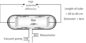 As the pressure inside the discharge tube is gradually reduced, the following is the sequence of phenomenon that are observed.
(1) At normal pressure no discharge takes place.
(2) At the pressure 10 mm of Hg, a zig-zag thin red spark runs from one electrode to other and cracking sound is heard.
As the pressure inside the discharge tube is gradually reduced, the following is the sequence of phenomenon that are observed.
(1) At normal pressure no discharge takes place.
(2) At the pressure 10 mm of Hg, a zig-zag thin red spark runs from one electrode to other and cracking sound is heard.
 (3) At the pressure 4 mm. of Hg, an illumination is observed at the electrodes and the rest of the tube appears dark. This type of discharge is called dark discharge.
(4) When the pressure falls below 4 mm of Hg then the whole tube is filled with bright light called positive column and colour of light depends upon the nature of gas in the tube as shown in the following table.
Colour for different gases
(3) At the pressure 4 mm. of Hg, an illumination is observed at the electrodes and the rest of the tube appears dark. This type of discharge is called dark discharge.
(4) When the pressure falls below 4 mm of Hg then the whole tube is filled with bright light called positive column and colour of light depends upon the nature of gas in the tube as shown in the following table.
Colour for different gases
| Gas | Air | \[{{H}_{2}}\] | \[{{N}_{2}}\] | \[C{{l}_{2}}\] | \[C{{O}_{2}}\] | Neon |
| Colour | Purple red | Blue | Red | Green | more...
Choke coil (or ballast) is a device having high inductance and negligible resistance. It is used to control current in ac circuits and is used in fluorescent tubes. The power loss in a circuit containing choke coil is least.
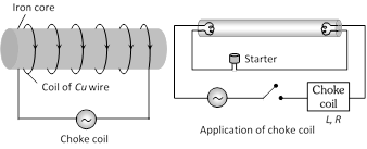 (1) It consist of a Cu coil wound over a soft iron laminated core.
(2) Thick Cu wire is used to reduce the resistance (R) of the circuit.
(3) Soft iron is used to improve inductance (L) of the circuit.
(4) The inductive reactance or effective opposition of the choke coil is given by \[{{X}_{L}}=\omega L=2\pi vL\]
(5) For an ideal choke coil \[r=0,\] no electric energy is wasted i.e. average power \[P=0\].
(6) In actual practice choke coil is equivalent to a \[R-L\] circuit.
(7) Choke coil for different frequencies are made by using different substances in their core.
For low frequency L should be large thus iron core choke coil is used. For high frequency ac circuit, L should be small, so air cored choke coil is used.
(1) It consist of a Cu coil wound over a soft iron laminated core.
(2) Thick Cu wire is used to reduce the resistance (R) of the circuit.
(3) Soft iron is used to improve inductance (L) of the circuit.
(4) The inductive reactance or effective opposition of the choke coil is given by \[{{X}_{L}}=\omega L=2\pi vL\]
(5) For an ideal choke coil \[r=0,\] no electric energy is wasted i.e. average power \[P=0\].
(6) In actual practice choke coil is equivalent to a \[R-L\] circuit.
(7) Choke coil for different frequencies are made by using different substances in their core.
For low frequency L should be large thus iron core choke coil is used. For high frequency ac circuit, L should be small, so air cored choke coil is used.
In an ac circuit \[R=0\]\[\Rightarrow \]\[\cos \phi =0\] so \[{{P}_{av}}=0\] i.e. in resistance less circuit the power consumed is zero. Such a circuit is called the wattless circuit and the current flowing is called the wattless current.
or
The component of current which does not contribute to the average power dissipation is called wattless current
(i) The average of wattless component over one cycle is zero
(ii) Amplitude of wattless current \[={{i}_{0}}\sin \phi \]
and r.m.s. value of wattless current\[={{i}_{rms}}\sin \varphi =\frac{{{i}_{0}}}{\sqrt{2}}\sin \phi \].
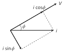 It is quadrature \[({{90}^{o}})\] with voltage.
\[{{i}_{R}}=\frac{{{V}_{0}}}{R}={{V}_{0}}G\]
\[{{i}_{L}}=\frac{{{V}_{0}}}{{{X}_{L}}}={{V}_{0}}{{S}_{L}}\]
\[{{i}_{C}}=\frac{{{V}_{0}}}{{{X}_{C}}}={{V}_{0}}{{S}_{C}}\]
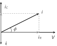
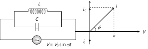
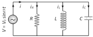 (1) Current and phase difference : From phasor diagram current \[i=\sqrt{i_{R}^{2}+{{({{i}_{C}}-{{i}_{L}})}^{2}}}\] and phase difference
\[\varphi ={{\tan }^{-1}}\frac{({{i}_{C}}-{{i}_{L}})}{{{i}_{R}}}={{\tan }^{-1}}\frac{({{S}_{C}}-{{S}_{L}})}{G}\]
(1) Current and phase difference : From phasor diagram current \[i=\sqrt{i_{R}^{2}+{{({{i}_{C}}-{{i}_{L}})}^{2}}}\] and phase difference
\[\varphi ={{\tan }^{-1}}\frac{({{i}_{C}}-{{i}_{L}})}{{{i}_{R}}}={{\tan }^{-1}}\frac{({{S}_{C}}-{{S}_{L}})}{G}\]
 (2) Admittance (Y) of the circuit : From equation of current \[\frac{{{V}_{0}}}{Z}=\sqrt{{{\left( \frac{{{V}_{0}}}{R} \right)}^{2}}+{{\left( \frac{{{V}_{0}}}{{{X}_{L}}}-\frac{{{V}_{0}}}{{{X}_{C}}} \right)}^{2}}}\]
\[\Rightarrow \]\[\frac{1}{Z}=Y=\sqrt{{{\left( \frac{1}{R} \right)}^{2}}+{{\left( \frac{1}{{{X}_{L}}}-\frac{1}{{{X}_{C}}} \right)}^{2}}}=\sqrt{{{G}^{2}}+{{({{S}_{L}}-{{S}_{C}})}^{2}}}\]
(3) Resonance : At resonance (i) \[{{i}_{C}}={{i}_{L}}\]\[\Rightarrow \]\[{{i}_{\min }}={{i}_{R}}\]
(ii) \[\frac{V}{{{X}_{C}}}=\frac{V}{{{X}_{L}}}\]\[\Rightarrow \]\[{{S}_{C}}={{S}_{L}}\,\Rightarrow \,\Sigma \,S=0\]
(iii) \[{{Z}_{\max }}=\frac{V}{{{i}_{R}}}=R\]
(iv) \[\varphi =0\]\[\Rightarrow \]\[\text{p}\text{.f}\text{.}\,\,=\cos \phi =1=\]maximum
(v) Resonant frequency \[\Rightarrow \nu =\frac{1}{2\pi \sqrt{LC}}\]
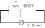
(4) Parallel LC circuits : If inductor has resistance (R) and it is connected in parallel with capacitor as shown
(i) At resonance
(2) Admittance (Y) of the circuit : From equation of current \[\frac{{{V}_{0}}}{Z}=\sqrt{{{\left( \frac{{{V}_{0}}}{R} \right)}^{2}}+{{\left( \frac{{{V}_{0}}}{{{X}_{L}}}-\frac{{{V}_{0}}}{{{X}_{C}}} \right)}^{2}}}\]
\[\Rightarrow \]\[\frac{1}{Z}=Y=\sqrt{{{\left( \frac{1}{R} \right)}^{2}}+{{\left( \frac{1}{{{X}_{L}}}-\frac{1}{{{X}_{C}}} \right)}^{2}}}=\sqrt{{{G}^{2}}+{{({{S}_{L}}-{{S}_{C}})}^{2}}}\]
(3) Resonance : At resonance (i) \[{{i}_{C}}={{i}_{L}}\]\[\Rightarrow \]\[{{i}_{\min }}={{i}_{R}}\]
(ii) \[\frac{V}{{{X}_{C}}}=\frac{V}{{{X}_{L}}}\]\[\Rightarrow \]\[{{S}_{C}}={{S}_{L}}\,\Rightarrow \,\Sigma \,S=0\]
(iii) \[{{Z}_{\max }}=\frac{V}{{{i}_{R}}}=R\]
(iv) \[\varphi =0\]\[\Rightarrow \]\[\text{p}\text{.f}\text{.}\,\,=\cos \phi =1=\]maximum
(v) Resonant frequency \[\Rightarrow \nu =\frac{1}{2\pi \sqrt{LC}}\]
(4) Parallel LC circuits : If inductor has resistance (R) and it is connected in parallel with capacitor as shown
(i) At resonance
 (a) \[{{Z}_{\max }}=\frac{1}{{{Y}_{\min }}}=\frac{L}{CR}\]
(b) Current through the circuit is minimum and \[{{i}_{\min }}=\frac{{{V}_{0}}CR}{L}\]
(c) \[{{S}_{L}}={{S}_{C}}\] \[\Rightarrow \]\[\frac{1}{{{X}_{L}}}=\frac{1}{{{X}_{C}}}\]\[\Rightarrow \]\[X=\infty \]
(d) Resonant frequency \[{{\omega }_{0}}=\sqrt{\frac{1}{LC}-\frac{{{R}^{2}}}{{{L}^{2}}}}\,\frac{rad}{sec}\] or \[{{\nu }_{0}}=\frac{1}{2\pi }\sqrt{\frac{1}{LC}-\frac{{{R}^{2}}}{{{L}^{2}}}}\,Hz\](Condition for parallel resonance is \[R<\sqrt{\frac{L}{C}}\])
(e) Quality factor of the circuit \[=\frac{1}{CR}.\frac{1}{\sqrt{\frac{1}{LC}-\frac{{{R}^{2}}}{{{L}^{2}}}}}\]. In the state of resonance the quality factor of the circuit is equivalent to the current amplification of the circuit.
(ii) If inductance has no resistance : If \[R=0\] then circuit becomes parallel LC circuit as shown
(a) \[{{Z}_{\max }}=\frac{1}{{{Y}_{\min }}}=\frac{L}{CR}\]
(b) Current through the circuit is minimum and \[{{i}_{\min }}=\frac{{{V}_{0}}CR}{L}\]
(c) \[{{S}_{L}}={{S}_{C}}\] \[\Rightarrow \]\[\frac{1}{{{X}_{L}}}=\frac{1}{{{X}_{C}}}\]\[\Rightarrow \]\[X=\infty \]
(d) Resonant frequency \[{{\omega }_{0}}=\sqrt{\frac{1}{LC}-\frac{{{R}^{2}}}{{{L}^{2}}}}\,\frac{rad}{sec}\] or \[{{\nu }_{0}}=\frac{1}{2\pi }\sqrt{\frac{1}{LC}-\frac{{{R}^{2}}}{{{L}^{2}}}}\,Hz\](Condition for parallel resonance is \[R<\sqrt{\frac{L}{C}}\])
(e) Quality factor of the circuit \[=\frac{1}{CR}.\frac{1}{\sqrt{\frac{1}{LC}-\frac{{{R}^{2}}}{{{L}^{2}}}}}\]. In the state of resonance the quality factor of the circuit is equivalent to the current amplification of the circuit.
(ii) If inductance has no resistance : If \[R=0\] then circuit becomes parallel LC circuit as shown
 Condition of resonance : \[{{i}_{C}}={{i}_{L}}\]\[\Rightarrow \]\[\frac{V}{{{X}_{C}}}=\frac{V}{{{X}_{L}}}\]
\[\Rightarrow \] \[{{X}_{C}}={{X}_{L}}\].
At resonance current \[i\] in the circuit is zero and impedance is infinite. Resonant frequency : \[{{\nu }_{0}}=\frac{1}{2\pi \sqrt{LC}}Hz\]
Condition of resonance : \[{{i}_{C}}={{i}_{L}}\]\[\Rightarrow \]\[\frac{V}{{{X}_{C}}}=\frac{V}{{{X}_{L}}}\]
\[\Rightarrow \] \[{{X}_{C}}={{X}_{L}}\].
At resonance current \[i\] in the circuit is zero and impedance is infinite. Resonant frequency : \[{{\nu }_{0}}=\frac{1}{2\pi \sqrt{LC}}Hz\] 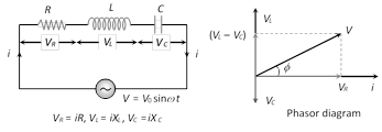 (1) Equation of current : \[i={{i}_{0}}\sin (\omega \,t\pm \varphi )\]; where \[{{i}_{0}}=\frac{{{V}_{0}}}{Z}\]
(2) Equation of voltage : From phasor diagram \[V=\sqrt{V_{R}^{2}+{{({{V}_{L}}-{{V}_{C}})}^{2}}}\]
(3) Impedance of the circuit : \[Z=\sqrt{{{R}^{2}}+{{({{X}_{L}}-{{X}_{C}})}^{2}}}=\sqrt{{{R}^{2}}+{{\left( \omega \,L-\frac{1}{\omega C} \right)}^{2}}}\]
(4) Phase difference : From phasor diagram \[\tan \varphi =\frac{{{V}_{L}}-{{V}_{C}}}{{{V}_{R}}}=\frac{{{X}_{L}}-{{X}_{C}}}{R}=\frac{\omega \,L-\frac{1}{\omega \,C}}{R}=\frac{2\pi \nu \,L-\frac{1}{2\pi \nu \,C}}{R}\]
(5) If net reactance is inductive : Circuit behaves as LR circuit
(6) If net reactance is capacitive : Circuit behave as CR circuit
(7) If net reactance is zero : Means \[X={{X}_{L}}-{{X}_{C}}=0\]
\[\Rightarrow \] \[{{X}_{L}}={{X}_{C}}\] . This is the condition of resonance
(8) At resonance (series resonant circuit)
(i) \[{{X}_{L}}={{X}_{C}}\Rightarrow {{Z}_{\min }}=R\] i.e. circuit behaves as resistive circuit
(ii) \[{{V}_{L}}={{V}_{C}}\Rightarrow V={{V}_{R}}\] i.e. whole applied voltage appeared across the resistance
(iii) Phase difference : \[\phi ={{0}^{o}}\]\[\Rightarrow \]\[p.f.\,=\cos \phi =1\]
(iv) Power consumption \[P={{V}_{rms}}\,{{i}_{rms}}=\frac{1}{2}{{V}_{0}}{{i}_{0}}\]
(v) Current in the circuit is maximum and it is \[{{i}_{0}}=\frac{{{V}_{0}}}{R}\]
(vi) These circuit are used for voltage amplification and as selector circuits in wireless telegraphy.
(9) Resonant frequency (Natural frequency)
At resonance \[{{X}_{L}}={{X}_{C}}\]\[\Rightarrow \] \[{{\omega }_{0}}L=\frac{1}{{{\omega }_{0}}C}\]\[\Rightarrow \]\[{{\omega }_{0}}=\frac{1}{\sqrt{LC}}\frac{rad}{sec}\]\[\Rightarrow \]\[{{\nu }_{0}}=\frac{1}{2\pi \sqrt{LC}}Hz\,(\text{or}\,cps)\]
(Resonant frequency doesn't depend upon the resistance of the circuit)
(10) Half power frequencies and band width : The frequencies at which the power in the circuit is half of the maximum power (The power at resonance), are called half power frequencies.
(i) The current in the circuit at half power frequencies (HPF) is \[\frac{1}{\sqrt{2}}\] or 0.707 or 70.7% of maximum current (current at resonance).
(1) Equation of current : \[i={{i}_{0}}\sin (\omega \,t\pm \varphi )\]; where \[{{i}_{0}}=\frac{{{V}_{0}}}{Z}\]
(2) Equation of voltage : From phasor diagram \[V=\sqrt{V_{R}^{2}+{{({{V}_{L}}-{{V}_{C}})}^{2}}}\]
(3) Impedance of the circuit : \[Z=\sqrt{{{R}^{2}}+{{({{X}_{L}}-{{X}_{C}})}^{2}}}=\sqrt{{{R}^{2}}+{{\left( \omega \,L-\frac{1}{\omega C} \right)}^{2}}}\]
(4) Phase difference : From phasor diagram \[\tan \varphi =\frac{{{V}_{L}}-{{V}_{C}}}{{{V}_{R}}}=\frac{{{X}_{L}}-{{X}_{C}}}{R}=\frac{\omega \,L-\frac{1}{\omega \,C}}{R}=\frac{2\pi \nu \,L-\frac{1}{2\pi \nu \,C}}{R}\]
(5) If net reactance is inductive : Circuit behaves as LR circuit
(6) If net reactance is capacitive : Circuit behave as CR circuit
(7) If net reactance is zero : Means \[X={{X}_{L}}-{{X}_{C}}=0\]
\[\Rightarrow \] \[{{X}_{L}}={{X}_{C}}\] . This is the condition of resonance
(8) At resonance (series resonant circuit)
(i) \[{{X}_{L}}={{X}_{C}}\Rightarrow {{Z}_{\min }}=R\] i.e. circuit behaves as resistive circuit
(ii) \[{{V}_{L}}={{V}_{C}}\Rightarrow V={{V}_{R}}\] i.e. whole applied voltage appeared across the resistance
(iii) Phase difference : \[\phi ={{0}^{o}}\]\[\Rightarrow \]\[p.f.\,=\cos \phi =1\]
(iv) Power consumption \[P={{V}_{rms}}\,{{i}_{rms}}=\frac{1}{2}{{V}_{0}}{{i}_{0}}\]
(v) Current in the circuit is maximum and it is \[{{i}_{0}}=\frac{{{V}_{0}}}{R}\]
(vi) These circuit are used for voltage amplification and as selector circuits in wireless telegraphy.
(9) Resonant frequency (Natural frequency)
At resonance \[{{X}_{L}}={{X}_{C}}\]\[\Rightarrow \] \[{{\omega }_{0}}L=\frac{1}{{{\omega }_{0}}C}\]\[\Rightarrow \]\[{{\omega }_{0}}=\frac{1}{\sqrt{LC}}\frac{rad}{sec}\]\[\Rightarrow \]\[{{\nu }_{0}}=\frac{1}{2\pi \sqrt{LC}}Hz\,(\text{or}\,cps)\]
(Resonant frequency doesn't depend upon the resistance of the circuit)
(10) Half power frequencies and band width : The frequencies at which the power in the circuit is half of the maximum power (The power at resonance), are called half power frequencies.
(i) The current in the circuit at half power frequencies (HPF) is \[\frac{1}{\sqrt{2}}\] or 0.707 or 70.7% of maximum current (current at resonance).
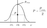 (ii) There are two half power frequencies
(a) \[{{\omega }_{1}}\to \] called lower half power frequency. At this frequency the circuit is capacitive.
(b) \[{{\omega }_{2}}\to \] called upper half power frequency. It is greater than \[{{\omega }_{0}}\]. At this frequency the circuit is inductive.
(iii) Band width \[(\Delta \omega )\]: The difference of half power frequencies \[{{\omega }_{1}}\] and \[{{\omega }_{2}}\] is called band width \[(\Delta \omega )\]and \[\Delta \omega ={{\omega }_{2}}-{{\omega }_{1}}\]. For series resonant circuit it can be proved \[\Delta \omega =\left( \frac{R}{L} \right)\]
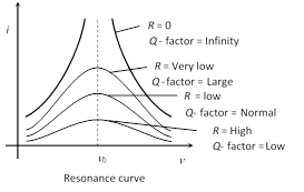
(11) Quality factor (Q-factor) of series resonant circuit
(i) The characteristic of a series resonant circuit is determined by the quality factor (Q - factor) of the circuit.
(ii) It defines sharpness of \[i-v\] curve at resonance when Q - factor is large, the sharpness of resonance curve is more and vice-versa.
(iii) Q - factor also defined as follows
Q - factor \[=2\pi \times \frac{\text{Max}\text{. energy stored}}{\text{Energy dissipation }}\]
\[=\frac{2\pi }{T}\times \frac{\text{Max}\text{. energy stored}}{\text{Mean power dissipated}}\]\[=\frac{\text{Resonant frequency}}{\text{Band width}}=\frac{{{\omega }_{0}}}{\Delta \omega }\]
(iv) Q - factor \[=\frac{{{V}_{L}}}{{{V}_{R}}}\] or \[\frac{{{V}_{C}}}{{{V}_{R}}}\]\[=\frac{{{\omega }_{0}}L}{R}\,\,\text{or}\,\,\frac{1}{{{\omega }_{0}}CR}\]
\[\Rightarrow Q\text{-factor}=\frac{1}{R}\sqrt{\frac{L}{C}}\]
(ii) There are two half power frequencies
(a) \[{{\omega }_{1}}\to \] called lower half power frequency. At this frequency the circuit is capacitive.
(b) \[{{\omega }_{2}}\to \] called upper half power frequency. It is greater than \[{{\omega }_{0}}\]. At this frequency the circuit is inductive.
(iii) Band width \[(\Delta \omega )\]: The difference of half power frequencies \[{{\omega }_{1}}\] and \[{{\omega }_{2}}\] is called band width \[(\Delta \omega )\]and \[\Delta \omega ={{\omega }_{2}}-{{\omega }_{1}}\]. For series resonant circuit it can be proved \[\Delta \omega =\left( \frac{R}{L} \right)\]
(11) Quality factor (Q-factor) of series resonant circuit
(i) The characteristic of a series resonant circuit is determined by the quality factor (Q - factor) of the circuit.
(ii) It defines sharpness of \[i-v\] curve at resonance when Q - factor is large, the sharpness of resonance curve is more and vice-versa.
(iii) Q - factor also defined as follows
Q - factor \[=2\pi \times \frac{\text{Max}\text{. energy stored}}{\text{Energy dissipation }}\]
\[=\frac{2\pi }{T}\times \frac{\text{Max}\text{. energy stored}}{\text{Mean power dissipated}}\]\[=\frac{\text{Resonant frequency}}{\text{Band width}}=\frac{{{\omega }_{0}}}{\Delta \omega }\]
(iv) Q - factor \[=\frac{{{V}_{L}}}{{{V}_{R}}}\] or \[\frac{{{V}_{C}}}{{{V}_{R}}}\]\[=\frac{{{\omega }_{0}}L}{R}\,\,\text{or}\,\,\frac{1}{{{\omega }_{0}}CR}\]
\[\Rightarrow Q\text{-factor}=\frac{1}{R}\sqrt{\frac{L}{C}}\]
  (1) Applied voltage : \[V={{V}_{L}}-{{V}_{C}}\]
(2) Impedance : \[Z={{X}_{L}}-{{X}_{C}}=X\]
(3) Current : \[i={{i}_{0}}\sin \,\left( \omega \,t\pm \frac{\pi }{2} \right)\]
(4) Peak current : \[{{i}_{0}}=\frac{{{V}_{0}}}{Z}=\frac{{{V}_{0}}}{{{X}_{L}}-{{X}_{C}}}\]\[=\frac{{{V}_{0}}}{\omega \,L-\frac{1}{\omega \,C}}\]
(5) Phase difference : \[\phi ={{90}^{o}}\]
(6) Power factor : \[\cos \varphi =0\]
(7) Leading quantity : Either voltage or current
(1) Applied voltage : \[V={{V}_{L}}-{{V}_{C}}\]
(2) Impedance : \[Z={{X}_{L}}-{{X}_{C}}=X\]
(3) Current : \[i={{i}_{0}}\sin \,\left( \omega \,t\pm \frac{\pi }{2} \right)\]
(4) Peak current : \[{{i}_{0}}=\frac{{{V}_{0}}}{Z}=\frac{{{V}_{0}}}{{{X}_{L}}-{{X}_{C}}}\]\[=\frac{{{V}_{0}}}{\omega \,L-\frac{1}{\omega \,C}}\]
(5) Phase difference : \[\phi ={{90}^{o}}\]
(6) Power factor : \[\cos \varphi =0\]
(7) Leading quantity : Either voltage or current 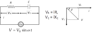 (1) Applied voltage : \[V=\sqrt{V_{R}^{2}+V_{C}^{2}}\]
(2) Impedance : \[Z=\sqrt{{{R}^{2}}+X_{C}^{2}}=\sqrt{{{R}^{2}}+{{\left( \frac{1}{\omega C} \right)}^{2}}}\]
(3) Current : \[i={{i}_{0}}\sin \,\left( \omega \,t+\varphi \right)\]
(4) Peak current : \[{{i}_{0}}=\frac{{{V}_{0}}}{Z}=\frac{{{V}_{0}}}{\sqrt{{{R}^{2}}+X_{C}^{2}}}\]\[=\frac{{{V}_{0}}}{\sqrt{{{R}^{2}}+\frac{1}{4{{\pi }^{2}}{{\nu }^{2}}{{C}^{2}}}}}\]
(5) Phase difference : \[\varphi ={{\tan }^{-1}}\frac{{{X}_{C}}}{R}={{\tan }^{-1}}\frac{1}{\omega CR}\]
(6) Power factor : \[\cos \varphi =\frac{R}{\sqrt{{{R}^{2}}+X_{C}^{2}}}\]
(7) Leading quantity : Current
(1) Applied voltage : \[V=\sqrt{V_{R}^{2}+V_{C}^{2}}\]
(2) Impedance : \[Z=\sqrt{{{R}^{2}}+X_{C}^{2}}=\sqrt{{{R}^{2}}+{{\left( \frac{1}{\omega C} \right)}^{2}}}\]
(3) Current : \[i={{i}_{0}}\sin \,\left( \omega \,t+\varphi \right)\]
(4) Peak current : \[{{i}_{0}}=\frac{{{V}_{0}}}{Z}=\frac{{{V}_{0}}}{\sqrt{{{R}^{2}}+X_{C}^{2}}}\]\[=\frac{{{V}_{0}}}{\sqrt{{{R}^{2}}+\frac{1}{4{{\pi }^{2}}{{\nu }^{2}}{{C}^{2}}}}}\]
(5) Phase difference : \[\varphi ={{\tan }^{-1}}\frac{{{X}_{C}}}{R}={{\tan }^{-1}}\frac{1}{\omega CR}\]
(6) Power factor : \[\cos \varphi =\frac{R}{\sqrt{{{R}^{2}}+X_{C}^{2}}}\]
(7) Leading quantity : Current Current Affairs CategoriesArchive
Trending Current Affairs


You need to login to perform this action. |

