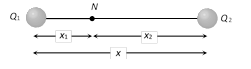
 If N is the neutral point at a distance \[{{x}_{1}}\] from \[{{Q}_{1}}\] and at a distance \[{{x}_{2}}\left( =x-{{x}_{1}} \right)\] from \[{{Q}_{2}}\] then
At N |E.F. due to \[{{\mathbf{Q}}_{\mathbf{1}}}\]| = |E.F. due to \[{{\mathbf{Q}}_{\mathbf{2}}}\]|
i.e., \[\frac{1}{4\pi {{\varepsilon }_{0}}}.\frac{{{Q}_{1}}}{x_{1}^{2}}=\frac{1}{4\pi {{\varepsilon }_{0}}}.\frac{{{Q}_{2}}}{x_{2}^{2}}\]\[\Rightarrow \]\[\frac{{{Q}_{1}}}{{{Q}_{2}}}={{\left( \frac{{{x}_{1}}}{{{x}_{2}}} \right)}^{2}}\]
Short Trick : \[{{x}_{1}}=\frac{x}{\sqrt{{{Q}_{2}}/{{Q}_{1}}}+1}\] and \[{{x}_{2}}=\frac{x}{\sqrt{{{Q}_{1}}/{{Q}_{2}}}+1}\]
(2) Neutral point due to a system of two unlike point charge : For this condition neutral point lies at an external point along the line joining two unlike charges. Suppose two unlike charge \[{{Q}_{1}}\] and \[{{Q}_{2}}\] separated by a distance \[x\] from each other.
If N is the neutral point at a distance \[{{x}_{1}}\] from \[{{Q}_{1}}\] and at a distance \[{{x}_{2}}\left( =x-{{x}_{1}} \right)\] from \[{{Q}_{2}}\] then
At N |E.F. due to \[{{\mathbf{Q}}_{\mathbf{1}}}\]| = |E.F. due to \[{{\mathbf{Q}}_{\mathbf{2}}}\]|
i.e., \[\frac{1}{4\pi {{\varepsilon }_{0}}}.\frac{{{Q}_{1}}}{x_{1}^{2}}=\frac{1}{4\pi {{\varepsilon }_{0}}}.\frac{{{Q}_{2}}}{x_{2}^{2}}\]\[\Rightarrow \]\[\frac{{{Q}_{1}}}{{{Q}_{2}}}={{\left( \frac{{{x}_{1}}}{{{x}_{2}}} \right)}^{2}}\]
Short Trick : \[{{x}_{1}}=\frac{x}{\sqrt{{{Q}_{2}}/{{Q}_{1}}}+1}\] and \[{{x}_{2}}=\frac{x}{\sqrt{{{Q}_{1}}/{{Q}_{2}}}+1}\]
(2) Neutral point due to a system of two unlike point charge : For this condition neutral point lies at an external point along the line joining two unlike charges. Suppose two unlike charge \[{{Q}_{1}}\] and \[{{Q}_{2}}\] separated by a distance \[x\] from each other.
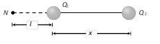 Here neutral point lies outside the line joining two unlike charges and also it lies nearer to charge which is smaller in magnitude.
If \[\left| \left. \,{{Q}_{\mathbf{1}}} \right| \right.<\left| \,\left. {{Q}_{\mathbf{2}}} \right| \right.\] then neutral point will be obtained on the side of \[{{Q}_{1}}\], suppose it is at a distance \[l\] from \[C=\frac{Q}{V}\]
so \[l=\frac{x}{\left( \sqrt{{{Q}_{\mathbf{2}}}/{{Q}_{\mathbf{1}}}}-\mathbf{1} \right)}\]
(3) Zero potential due to a system of two point charge
(i) If both charges are like then resultant potential is not zero at any finite point.
(ii) If the charges are unequal and unlike then all such points where resultant potential is zero lies on a closed curve.
(iii) Along the line joining the two charge, two such points exist, one lies inside and one lies outside the charges on the line joining the charges. Both the above points lie nearer the smaller charge.
For internal point
(It is assumed that \[|{{Q}_{1}}\,|\,<\,|{{Q}_{2}}|\]).
Here neutral point lies outside the line joining two unlike charges and also it lies nearer to charge which is smaller in magnitude.
If \[\left| \left. \,{{Q}_{\mathbf{1}}} \right| \right.<\left| \,\left. {{Q}_{\mathbf{2}}} \right| \right.\] then neutral point will be obtained on the side of \[{{Q}_{1}}\], suppose it is at a distance \[l\] from \[C=\frac{Q}{V}\]
so \[l=\frac{x}{\left( \sqrt{{{Q}_{\mathbf{2}}}/{{Q}_{\mathbf{1}}}}-\mathbf{1} \right)}\]
(3) Zero potential due to a system of two point charge
(i) If both charges are like then resultant potential is not zero at any finite point.
(ii) If the charges are unequal and unlike then all such points where resultant potential is zero lies on a closed curve.
(iii) Along the line joining the two charge, two such points exist, one lies inside and one lies outside the charges on the line joining the charges. Both the above points lie nearer the smaller charge.
For internal point
(It is assumed that \[|{{Q}_{1}}\,|\,<\,|{{Q}_{2}}|\]).
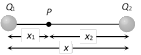 At P, \[\frac{{{Q}_{1}}}{{{x}_{1}}}=\frac{{{Q}_{2}}}{\left( x-{{x}_{1}} \right)}\]
\[\Rightarrow \] \[{{x}_{1}}=\frac{x}{\left( {{Q}_{2}}/{{Q}_{\mathbf{1}}}+1 \right)}\]
For External point
At P, \[\frac{{{Q}_{1}}}{{{x}_{1}}}=\frac{{{Q}_{2}}}{\left( x-{{x}_{1}} \right)}\]
\[\Rightarrow \] \[{{x}_{1}}=\frac{x}{\left( {{Q}_{2}}/{{Q}_{\mathbf{1}}}+1 \right)}\]
For External point
 At P, \[\frac{{{Q}_{1}}}{{{x}_{1}}}=\frac{{{Q}_{2}}}{\left( x+{{x}_{1}} \right)}\]
\[\Rightarrow \] \[{{x}_{1}}=\frac{x}{\left( {{Q}_{2}}/{{Q}_{\mathbf{1}}}-1 \right)}\]
At P, \[\frac{{{Q}_{1}}}{{{x}_{1}}}=\frac{{{Q}_{2}}}{\left( x+{{x}_{1}} \right)}\]
\[\Rightarrow \] \[{{x}_{1}}=\frac{x}{\left( {{Q}_{2}}/{{Q}_{\mathbf{1}}}-1 \right)}\]  Case-1 : If some charge say +Q is given to bob and an electric field E is applied in the direction as shown in figure then equilibrium position of charged bob (point charge) changes from O to O'.
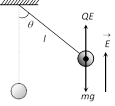
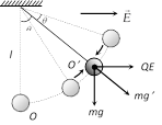 On displacing the bob from it's equilibrium position 0 it will oscillate under the effective acceleration g', where
\[mg'=\sqrt{{{\left( mg \right)}^{2}}+{{\left( QE \right)}^{2}}}\] \[\Rightarrow g'=\sqrt{{{g}^{2}}+{{\left( QE/m \right)}^{2}}}\].
Hence the new time period is \[{{T}_{1}}=2\pi \sqrt{\frac{l}{g'}}\]\[=2\pi \sqrt{\frac{l}{\left( {{g}^{2}}+\left( QE/m \right){{\,}^{2}} \right){{\,}^{\frac{1}{2}}}}}\]
Since \[g'>g,\] so \[{{T}_{1}}<T\] i.e. time period of pendulum will decrease.
Case-2 : If electric field is applied in the downward direction then. Effective acceleration
On displacing the bob from it's equilibrium position 0 it will oscillate under the effective acceleration g', where
\[mg'=\sqrt{{{\left( mg \right)}^{2}}+{{\left( QE \right)}^{2}}}\] \[\Rightarrow g'=\sqrt{{{g}^{2}}+{{\left( QE/m \right)}^{2}}}\].
Hence the new time period is \[{{T}_{1}}=2\pi \sqrt{\frac{l}{g'}}\]\[=2\pi \sqrt{\frac{l}{\left( {{g}^{2}}+\left( QE/m \right){{\,}^{2}} \right){{\,}^{\frac{1}{2}}}}}\]
Since \[g'>g,\] so \[{{T}_{1}}<T\] i.e. time period of pendulum will decrease.
Case-2 : If electric field is applied in the downward direction then. Effective acceleration
 \[g'=g+QE/m\]
So new time period
\[{{T}_{2}}=2\pi \sqrt{\frac{l}{g+\left( QE/m \right)}}\]
\[{{T}_{2}}<T\]
Case-3 : In case 2 if electric field is applied in upward direction then, effective acceleration.
\[g'=g-QE/m\]
\[g'=g+QE/m\]
So new time period
\[{{T}_{2}}=2\pi \sqrt{\frac{l}{g+\left( QE/m \right)}}\]
\[{{T}_{2}}<T\]
Case-3 : In case 2 if electric field is applied in upward direction then, effective acceleration.
\[g'=g-QE/m\]
 So new time period
\[{{T}_{3}}=2\pi \sqrt{\frac{l}{g-\left( QE/m \right)}}\]
\[{{T}_{3}}>T\]
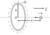
(2) Charged circular ring : A thin stationary ring of radius R has a positive charge +Q unit. If a negative charge \[-q\] (mass m) is placed at a small distance \[x\] from the centre. Then motion of the particle will be simple harmonic motion.
Having time period \[T=2\pi \sqrt{\frac{4\pi {{\varepsilon }_{0}}m{{R}^{3}}}{Q\,q}}\]
So new time period
\[{{T}_{3}}=2\pi \sqrt{\frac{l}{g-\left( QE/m \right)}}\]
\[{{T}_{3}}>T\]
(2) Charged circular ring : A thin stationary ring of radius R has a positive charge +Q unit. If a negative charge \[-q\] (mass m) is placed at a small distance \[x\] from the centre. Then motion of the particle will be simple harmonic motion.
Having time period \[T=2\pi \sqrt{\frac{4\pi {{\varepsilon }_{0}}m{{R}^{3}}}{Q\,q}}\]
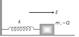
 (3) Spring mass system : A block of mass m containing a negative charge \[-Q\] is placed on a frictionless horizontal table and is connected to a wall through an unstretched spring of spring constant k as shown. If electric field E applied as shown in figure the block experiences an electric force, hence spring compress and block comes in new position. This is called the equilibrium position of block under the influence of electric field. If block compressed further or stretched, it execute oscillation having time period
\[T=2\pi \sqrt{\frac{m}{k}}\].
Maximum compression in the spring due to electric field \[=\frac{QE}{k}\]
(3) Spring mass system : A block of mass m containing a negative charge \[-Q\] is placed on a frictionless horizontal table and is connected to a wall through an unstretched spring of spring constant k as shown. If electric field E applied as shown in figure the block experiences an electric force, hence spring compress and block comes in new position. This is called the equilibrium position of block under the influence of electric field. If block compressed further or stretched, it execute oscillation having time period
\[T=2\pi \sqrt{\frac{m}{k}}\].
Maximum compression in the spring due to electric field \[=\frac{QE}{k}\]
| Suspended charge | System of three collinear charge |
Freely suspended charge
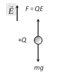 In equilibrium
\[QE=mg\]
\[\Rightarrow E=\frac{mg}{Q}\]
Suspension of charge from string
In equilibrium
\[QE=mg\]
\[\Rightarrow E=\frac{mg}{Q}\]
Suspension of charge from string
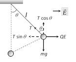 In equilibrium
\[T\sin \theta =QE\] ...(i)
\[T\cos \theta =mg\] ...(ii)
From equations (i) and (ii)
\[T=\sqrt{{{\left( QE \right)}^{2}}+{{\left( mg \right)}^{2}}}\]
and \[\tan \theta =\frac{QE}{mg}\]
In equilibrium
\[T\sin \theta =QE\] ...(i)
\[T\cos \theta =mg\] ...(ii)
From equations (i) and (ii)
\[T=\sqrt{{{\left( QE \right)}^{2}}+{{\left( mg \right)}^{2}}}\]
and \[\tan \theta =\frac{QE}{mg}\]
|
In the following figure three charges \[{{Q}_{1}},\,Q\] and \[{{Q}_{2}}\] are kept along a straight line, charge Q will be in equilibrium if and only if
|Force applied by charge \[{{Q}_{1}}\]|
= |Force applied by charge \[{{Q}_{2}}\]|
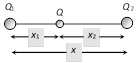 i.e. \[\frac{{{Q}_{1}}Q}{x_{1}^{2}}=\frac{{{Q}_{2}}Q}{x_{2}^{2}}\]
\[\Rightarrow \frac{{{Q}_{1}}}{{{Q}_{2}}}={{\left( \frac{{{x}_{1}}}{{{x}_{2}}} \right)}^{2}}\]
This is the necessary condition for Q to be in equilibrium. If all the three charges (\[{{Q}_{1}},\,Q\] and \[{{Q}_{2}}\]) are similar, Q will be in stable equilibrium.
If extreme charges are similar while charge Q is of different nature so Q will be in unstable equilibrium.
i.e. \[\frac{{{Q}_{1}}Q}{x_{1}^{2}}=\frac{{{Q}_{2}}Q}{x_{2}^{2}}\]
\[\Rightarrow \frac{{{Q}_{1}}}{{{Q}_{2}}}={{\left( \frac{{{x}_{1}}}{{{x}_{2}}} \right)}^{2}}\]
This is the necessary condition for Q to be in equilibrium. If all the three charges (\[{{Q}_{1}},\,Q\] and \[{{Q}_{2}}\]) are similar, Q will be in stable equilibrium.
If extreme charges are similar while charge Q is of different nature so Q will be in unstable equilibrium.
|
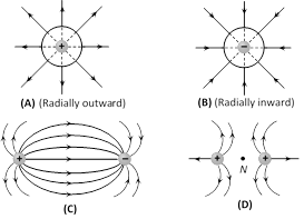 (2) Properties of electric lines of force
(i) Electric field lines come out of positive charge and go into the negative charge.
(ii) Tangent to the field line at any point gives the direction of the field at that point.
(2) Properties of electric lines of force
(i) Electric field lines come out of positive charge and go into the negative charge.
(ii) Tangent to the field line at any point gives the direction of the field at that point.
 (iii) Field lines never intersect each other.
(iv) Field lines are always normal to conducting surface.
(iii) Field lines never intersect each other.
(iv) Field lines are always normal to conducting surface.
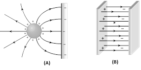 (v) Field lines do not exist inside a conductor.
(vi) The electric field lines never form closed loops. (While magnetic lines of forces form closed loop)
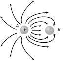
(vii) The number of lines originating or terminating on a charge is proportional to the magnitude of charge i.e. \[|Q|\,\,\propto \] number of lines. In the following figure \[|{{Q}_{A}}|\,>\,|{{Q}_{B}}|\]
(v) Field lines do not exist inside a conductor.
(vi) The electric field lines never form closed loops. (While magnetic lines of forces form closed loop)
(vii) The number of lines originating or terminating on a charge is proportional to the magnitude of charge i.e. \[|Q|\,\,\propto \] number of lines. In the following figure \[|{{Q}_{A}}|\,>\,|{{Q}_{B}}|\]
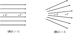
 (viii) If the lines of forces are equidistant and parallel straight lines the field is uniform and if either lines of force are not equidistant or straight line or both the field will be non uniform, also the density of field lines is proportional to the strength of the electric field.
 (iii) Momentum : Momentum\[p=mv,\,\,p=m\times \frac{QEt}{m}=QEt\]
or \[p=m\times \sqrt{\frac{2Q\Delta V}{m}}=\sqrt{2mQ\Delta V}\]
(iv) Kinetic energy : Kinetic energy gained by the particle in time t is \[K=\frac{1}{2}m{{v}^{2}}=\frac{1}{2}m{{\left( \frac{QEt}{m} \right)}^{2}}=\frac{{{Q}^{2}}{{E}^{2}}{{t}^{2}}}{2m}\]
or \[K=\frac{1}{2}m\times \frac{2QV}{m}=Q\Delta V\]
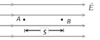
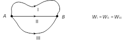
(v) Work done : According to work energy theorem we can say that gain in kinetic energy = work done in displacement of charge i.e. \[W=Q\Delta V\]
where \[\Delta V=\] Potential difference between the two position of charge Q. (\[\Delta V=\overrightarrow{E\,}.\Delta \overrightarrow{\,r\,}=E\Delta r\,\cos \theta \] where \[\theta \] is the angle between direction of electric field and direction of motion of charge).
If charge Q is given a displacement \[\overrightarrow{\,r\,}=({{r}_{1}}\hat{i}+{{r}_{2}}\hat{j}+{{r}_{3}}\hat{k})\] in an electric field \[\overrightarrow{\,E\,}=({{E}_{1}}\hat{i}+{{E}_{2}}\hat{j}+{{E}_{3}}\hat{k}).\] the work done is \[W=Q(\overrightarrow{\,E\,}.\overrightarrow{\,r\,})=Q({{E}_{1}}{{r}_{1}}+{{E}_{2}}{{r}_{2}}+{{E}_{3}}{{r}_{3}})\].
Work done in displacing a charge in an electric field is path independent.
(iii) Momentum : Momentum\[p=mv,\,\,p=m\times \frac{QEt}{m}=QEt\]
or \[p=m\times \sqrt{\frac{2Q\Delta V}{m}}=\sqrt{2mQ\Delta V}\]
(iv) Kinetic energy : Kinetic energy gained by the particle in time t is \[K=\frac{1}{2}m{{v}^{2}}=\frac{1}{2}m{{\left( \frac{QEt}{m} \right)}^{2}}=\frac{{{Q}^{2}}{{E}^{2}}{{t}^{2}}}{2m}\]
or \[K=\frac{1}{2}m\times \frac{2QV}{m}=Q\Delta V\]
(v) Work done : According to work energy theorem we can say that gain in kinetic energy = work done in displacement of charge i.e. \[W=Q\Delta V\]
where \[\Delta V=\] Potential difference between the two position of charge Q. (\[\Delta V=\overrightarrow{E\,}.\Delta \overrightarrow{\,r\,}=E\Delta r\,\cos \theta \] where \[\theta \] is the angle between direction of electric field and direction of motion of charge).
If charge Q is given a displacement \[\overrightarrow{\,r\,}=({{r}_{1}}\hat{i}+{{r}_{2}}\hat{j}+{{r}_{3}}\hat{k})\] in an electric field \[\overrightarrow{\,E\,}=({{E}_{1}}\hat{i}+{{E}_{2}}\hat{j}+{{E}_{3}}\hat{k}).\] the work done is \[W=Q(\overrightarrow{\,E\,}.\overrightarrow{\,r\,})=Q({{E}_{1}}{{r}_{1}}+{{E}_{2}}{{r}_{2}}+{{E}_{3}}{{r}_{3}})\].
Work done in displacing a charge in an electric field is path independent.
 (2) When a charged particle enters with an initial velocity at right angle to the uniform field
When charged particle enters perpendicularly in an electric field, it describe a parabolic path as shown
(i) Equation of trajectory : Throughout the motion particle has uniform velocity along x-axis and horizontal displacement (x) is given by the equation \[x=ut\]
Since the motion of the particle is accelerated along y-axis
(2) When a charged particle enters with an initial velocity at right angle to the uniform field
When charged particle enters perpendicularly in an electric field, it describe a parabolic path as shown
(i) Equation of trajectory : Throughout the motion particle has uniform velocity along x-axis and horizontal displacement (x) is given by the equation \[x=ut\]
Since the motion of the particle is accelerated along y-axis
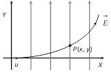 So \[y=\frac{1}{2}\left( \frac{QE}{m} \right)\,{{\left( \frac{x}{u} \right)}^{2}}\]; this is the equation of parabola which shows \[y\propto {{x}^{2}}\]
(ii) Velocity at any instant : At any instant t, \[{{v}_{x}}=u\] and \[{{v}_{y}}=\frac{QEt}{m}\] so \[v=\,|\overrightarrow{\,v}|\,=\sqrt{v_{x}^{2}+v_{y}^{2}}=\sqrt{{{u}^{2}}+\frac{{{Q}^{2}}{{E}^{2}}{{t}^{2}}}{{{m}^{2}}}}\]
If \[\beta \] is the angle made by v with x-axis than \[\tan \beta =\frac{{{v}_{y}}}{{{v}_{x}}}=\frac{QEt}{mu}\].
So \[y=\frac{1}{2}\left( \frac{QE}{m} \right)\,{{\left( \frac{x}{u} \right)}^{2}}\]; this is the equation of parabola which shows \[y\propto {{x}^{2}}\]
(ii) Velocity at any instant : At any instant t, \[{{v}_{x}}=u\] and \[{{v}_{y}}=\frac{QEt}{m}\] so \[v=\,|\overrightarrow{\,v}|\,=\sqrt{v_{x}^{2}+v_{y}^{2}}=\sqrt{{{u}^{2}}+\frac{{{Q}^{2}}{{E}^{2}}{{t}^{2}}}{{{m}^{2}}}}\]
If \[\beta \] is the angle made by v with x-axis than \[\tan \beta =\frac{{{v}_{y}}}{{{v}_{x}}}=\frac{QEt}{mu}\].

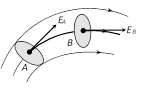
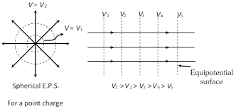 (4) For a uniform electric field, the equipotential surfaces are a family of plane perpendicular to the field lines.
(5) A metallic surface of any shape is an equipotential surface.
(6) Equipotential surfaces can never cross each other.
(7) The work done in moving a charge along an equipotential surface is always zero.
(4) For a uniform electric field, the equipotential surfaces are a family of plane perpendicular to the field lines.
(5) A metallic surface of any shape is an equipotential surface.
(6) Equipotential surfaces can never cross each other.
(7) The work done in moving a charge along an equipotential surface is always zero. 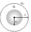 \[{{V}_{1}}=\frac{1}{4\pi {{\varepsilon }_{0}}}.\frac{{{Q}_{1}}}{{{r}_{1}}}+\frac{1}{4\pi {{\varepsilon }_{0}}}.\frac{{{Q}_{2}}}{{{r}_{2}}}\]
\[{{V}_{2}}=\frac{1}{4\pi {{\varepsilon }_{0}}}.\frac{{{Q}_{1}}}{{{r}_{2}}}+\frac{1}{4\pi {{\varepsilon }_{0}}}.\frac{{{Q}_{2}}}{{{r}_{2}}}\]
(2) The figure shows three conducting concentric shell of radii \[a,\,\,b\] and \[c(a<b<c)\] having charges \[{{Q}_{a}},\,{{Q}_{b}}\] and \[{{Q}_{c}}\] respectively
\[{{V}_{1}}=\frac{1}{4\pi {{\varepsilon }_{0}}}.\frac{{{Q}_{1}}}{{{r}_{1}}}+\frac{1}{4\pi {{\varepsilon }_{0}}}.\frac{{{Q}_{2}}}{{{r}_{2}}}\]
\[{{V}_{2}}=\frac{1}{4\pi {{\varepsilon }_{0}}}.\frac{{{Q}_{1}}}{{{r}_{2}}}+\frac{1}{4\pi {{\varepsilon }_{0}}}.\frac{{{Q}_{2}}}{{{r}_{2}}}\]
(2) The figure shows three conducting concentric shell of radii \[a,\,\,b\] and \[c(a<b<c)\] having charges \[{{Q}_{a}},\,{{Q}_{b}}\] and \[{{Q}_{c}}\] respectively 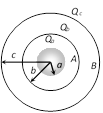 Potential at A;
\[{{V}_{A}}=\frac{1}{4\pi {{\varepsilon }_{0}}}\left[ \frac{{{Q}_{a}}}{a}+\frac{{{Q}_{b}}}{b}+\frac{{{Q}_{c}}}{c} \right]\]
Potential at B;
\[{{V}_{B}}=\frac{1}{4\pi {{\varepsilon }_{0}}}\left[ \frac{{{Q}_{a}}}{b}+\frac{{{Q}_{b}}}{b}+\frac{{{Q}_{c}}}{c} \right]\]
Potential at C;
\[{{V}_{C}}=\frac{1}{4\pi {{\varepsilon }_{0}}}\left[ \frac{{{Q}_{a}}}{c}+\frac{{{Q}_{b}}}{c}+\frac{{{Q}_{c}}}{c} \right]\]
(3) The figure shows two concentric spheres having radii \[{{r}_{1}}\] and \[{{r}_{2}}\] respectively \[({{r}_{2}}>{{r}_{1}})\]. If charge on inner sphere is +Q and outer sphere is earthed then
Potential at A;
\[{{V}_{A}}=\frac{1}{4\pi {{\varepsilon }_{0}}}\left[ \frac{{{Q}_{a}}}{a}+\frac{{{Q}_{b}}}{b}+\frac{{{Q}_{c}}}{c} \right]\]
Potential at B;
\[{{V}_{B}}=\frac{1}{4\pi {{\varepsilon }_{0}}}\left[ \frac{{{Q}_{a}}}{b}+\frac{{{Q}_{b}}}{b}+\frac{{{Q}_{c}}}{c} \right]\]
Potential at C;
\[{{V}_{C}}=\frac{1}{4\pi {{\varepsilon }_{0}}}\left[ \frac{{{Q}_{a}}}{c}+\frac{{{Q}_{b}}}{c}+\frac{{{Q}_{c}}}{c} \right]\]
(3) The figure shows two concentric spheres having radii \[{{r}_{1}}\] and \[{{r}_{2}}\] respectively \[({{r}_{2}}>{{r}_{1}})\]. If charge on inner sphere is +Q and outer sphere is earthed then
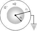 (i) Potential at the surface of outer sphere
\[{{V}_{2}}=\frac{1}{4\pi {{\varepsilon }_{0}}}.\frac{Q}{{{r}_{2}}}+\frac{1}{4\pi {{\varepsilon }_{0}}}.\frac{Q'}{{{r}_{2}}}=0\]
\[\Rightarrow \] \[Q'=-Q\]
(ii) Potential of the inner sphere
\[{{V}_{1}}=\frac{1}{4\pi {{\varepsilon }_{0}}}.\frac{Q}{{{r}_{1}}}+\frac{1}{4\pi {{\varepsilon }_{0}}}\,\frac{(-Q)}{{{r}_{2}}}\]\[=\frac{Q}{4\pi {{\varepsilon }_{0}}}\left[ \frac{1}{{{r}_{1}}}-\frac{1}{{{r}_{2}}} \right]\]
(4) In the above case if outer sphere is given a charge +Q and inner sphere is earthed then
(i) In this case potential at the surface of inner sphere is zero, so if \[Q'\] is the charge induced on inner sphere
then \[{{V}_{1}}=\frac{1}{4\pi {{\varepsilon }_{0}}}\left[ \frac{Q'}{{{r}_{1}}}+\frac{Q}{{{r}_{2}}} \right]=0\]
i.e., \[Q'=-\frac{{{r}_{1}}}{{{r}_{2}}}Q\]
(i) Potential at the surface of outer sphere
\[{{V}_{2}}=\frac{1}{4\pi {{\varepsilon }_{0}}}.\frac{Q}{{{r}_{2}}}+\frac{1}{4\pi {{\varepsilon }_{0}}}.\frac{Q'}{{{r}_{2}}}=0\]
\[\Rightarrow \] \[Q'=-Q\]
(ii) Potential of the inner sphere
\[{{V}_{1}}=\frac{1}{4\pi {{\varepsilon }_{0}}}.\frac{Q}{{{r}_{1}}}+\frac{1}{4\pi {{\varepsilon }_{0}}}\,\frac{(-Q)}{{{r}_{2}}}\]\[=\frac{Q}{4\pi {{\varepsilon }_{0}}}\left[ \frac{1}{{{r}_{1}}}-\frac{1}{{{r}_{2}}} \right]\]
(4) In the above case if outer sphere is given a charge +Q and inner sphere is earthed then
(i) In this case potential at the surface of inner sphere is zero, so if \[Q'\] is the charge induced on inner sphere
then \[{{V}_{1}}=\frac{1}{4\pi {{\varepsilon }_{0}}}\left[ \frac{Q'}{{{r}_{1}}}+\frac{Q}{{{r}_{2}}} \right]=0\]
i.e., \[Q'=-\frac{{{r}_{1}}}{{{r}_{2}}}Q\]
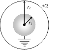 (Charge on inner sphere is less than that of the outer sphere.)
(ii) Potential at the surface of outer sphere
\[{{V}_{2}}=\frac{1}{4\pi {{\varepsilon }_{0}}}.\frac{Q'}{{{r}_{2}}}+\frac{1}{4\pi {{\varepsilon }_{0}}}.\frac{Q}{{{r}_{2}}}\]
\[{{V}_{2}}=\frac{1}{4\pi {{\varepsilon }_{0}}{{r}_{2}}}\left[ -Q\frac{{{r}_{1}}}{{{r}_{2}}}+Q \right]\] \[=\frac{Q}{4\pi {{\varepsilon }_{0}}{{r}_{2}}}\left[ 1-\frac{{{r}_{1}}}{{{r}_{2}}} \right]\]
(Charge on inner sphere is less than that of the outer sphere.)
(ii) Potential at the surface of outer sphere
\[{{V}_{2}}=\frac{1}{4\pi {{\varepsilon }_{0}}}.\frac{Q'}{{{r}_{2}}}+\frac{1}{4\pi {{\varepsilon }_{0}}}.\frac{Q}{{{r}_{2}}}\]
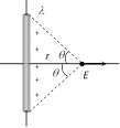
\[{{V}_{2}}=\frac{1}{4\pi {{\varepsilon }_{0}}{{r}_{2}}}\left[ -Q\frac{{{r}_{1}}}{{{r}_{2}}}+Q \right]\] \[=\frac{Q}{4\pi {{\varepsilon }_{0}}{{r}_{2}}}\left[ 1-\frac{{{r}_{1}}}{{{r}_{2}}} \right]\] 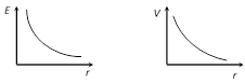 (2) Line charge: Electric field and potential due to a charged straight conducting wire of length \[l\] and charge density\[\lambda \]
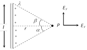 \[{{E}_{x}}=\frac{k\lambda }{r}(\sin \alpha +\sin \beta )\] and \[{{E}_{y}}=\frac{k\lambda }{r}(\cos \beta -\cos \alpha )\]
\[V=\frac{\lambda }{2\pi {{\varepsilon }_{0}}}{{\log }_{e}}\,\left[ \frac{\sqrt{{{r}^{2}}+{{l}^{2}}}-l}{\sqrt{{{r}^{2}}+{{l}^{2}}}+l} \right]\]
(i) If point P lies at perpendicular bisector of wire i.e. \[\alpha =\beta ;\,\,{{E}_{x}}=\frac{2k\lambda }{r}\sin \alpha \] and \[{{E}_{y}}=0\]
(ii) If wire is infinitely long i.e. \[l\to \infty \] so \[\alpha =\beta =\frac{\pi }{2};\,{{E}_{x}}=\frac{2k\lambda }{r}\] and \[{{E}_{y}}=0\Rightarrow {{E}_{net}}=\frac{\lambda }{2\pi {{\varepsilon }_{0}}r}\] and \[V=\frac{-\lambda }{2\pi {{\varepsilon }_{0}}}{{\log }_{e}}r+c\]
(iii) If point P lies near one end of infinitely long wire i.e. \[\alpha =0,\,\] and \[\beta =\frac{\pi }{2}\]
\[{{E}_{x}}=\frac{k\lambda }{r}(\sin \alpha +\sin \beta )\] and \[{{E}_{y}}=\frac{k\lambda }{r}(\cos \beta -\cos \alpha )\]
\[V=\frac{\lambda }{2\pi {{\varepsilon }_{0}}}{{\log }_{e}}\,\left[ \frac{\sqrt{{{r}^{2}}+{{l}^{2}}}-l}{\sqrt{{{r}^{2}}+{{l}^{2}}}+l} \right]\]
(i) If point P lies at perpendicular bisector of wire i.e. \[\alpha =\beta ;\,\,{{E}_{x}}=\frac{2k\lambda }{r}\sin \alpha \] and \[{{E}_{y}}=0\]
(ii) If wire is infinitely long i.e. \[l\to \infty \] so \[\alpha =\beta =\frac{\pi }{2};\,{{E}_{x}}=\frac{2k\lambda }{r}\] and \[{{E}_{y}}=0\Rightarrow {{E}_{net}}=\frac{\lambda }{2\pi {{\varepsilon }_{0}}r}\] and \[V=\frac{-\lambda }{2\pi {{\varepsilon }_{0}}}{{\log }_{e}}r+c\]
(iii) If point P lies near one end of infinitely long wire i.e. \[\alpha =0,\,\] and \[\beta =\frac{\pi }{2}\]
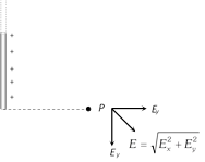 \[|{{E}_{x}}|\,=\,|{{E}_{y}}|\,=\frac{k\lambda }{r}\]
\[\Rightarrow \] \[{{E}_{net}}=\sqrt{E_{x}^{2}+E_{y}^{2}}=\frac{\sqrt{2}\,k\lambda }{r}\]
(3) Charged circular ring : Suppose we have a charged circular ring of radius R and charge Q. On it's axis electric field and potential is to be determined, at a point 'x' distance away from the centre of the ring.
\[|{{E}_{x}}|\,=\,|{{E}_{y}}|\,=\frac{k\lambda }{r}\]
\[\Rightarrow \] \[{{E}_{net}}=\sqrt{E_{x}^{2}+E_{y}^{2}}=\frac{\sqrt{2}\,k\lambda }{r}\]
(3) Charged circular ring : Suppose we have a charged circular ring of radius R and charge Q. On it's axis electric field and potential is to be determined, at a point 'x' distance away from the centre of the ring.
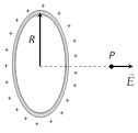 At point P
\[E=\frac{k\,Q\,x}{{{({{x}^{2}}+{{R}^{2}})}^{3/2}}},\]\[V=\frac{k\,Q}{\sqrt{{{x}^{2}}+{{R}^{2}}}}\]
At centre \[x=0\] so \[{{E}_{centre}}=0\] and \[{{V}_{centre}}=\frac{kQ}{R}\]
At a point on the axis such that \[x>>R\] \[E=\frac{kQ}{{{x}^{2}}}\], \[V=\frac{kQ}{x}\]
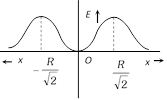
If \[x=\pm \frac{R}{\sqrt{2}}\], \[{{E}_{\max }}=\frac{Q}{6\sqrt{3}\pi {{\varepsilon }_{0}}{{a}^{2}}}\] and \[{{V}_{\max }}=\frac{Q}{2\sqrt{6}\pi {{\varepsilon }_{0}}}\]
Graph
At point P
\[E=\frac{k\,Q\,x}{{{({{x}^{2}}+{{R}^{2}})}^{3/2}}},\]\[V=\frac{k\,Q}{\sqrt{{{x}^{2}}+{{R}^{2}}}}\]
At centre \[x=0\] so \[{{E}_{centre}}=0\] and \[{{V}_{centre}}=\frac{kQ}{R}\]
At a point on the axis such that \[x>>R\] \[E=\frac{kQ}{{{x}^{2}}}\], \[V=\frac{kQ}{x}\]
If \[x=\pm \frac{R}{\sqrt{2}}\], \[{{E}_{\max }}=\frac{Q}{6\sqrt{3}\pi {{\varepsilon }_{0}}{{a}^{2}}}\] and \[{{V}_{\max }}=\frac{Q}{2\sqrt{6}\pi {{\varepsilon }_{0}}}\]
Graph
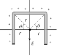
 (4) Some more results of line charge : If a thin plastic rod having charge density \[\lambda \] is bent in the following shapes then electric field at P in different situations shown in the following table Bending of charged rod
 \[E=\frac{2k\lambda }{r}\sin \theta \]
|
 \[E=\frac{2k\lambda }{r}\cos \theta \]
|
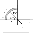 \[E=\frac{\sqrt{2}\,k\lambda }{r}\]
|
 \[E=\frac{2k\lambda }{r}\]
|
 more... more...
(1) Definition : Potential at a point in a field is defined as the amount of work done in bringing a unit positive test charge, from infinity to that point along any arbitrary path (infinity is point of zero potential). Electric potential is a scalar quantity, it is denoted by V; \[V=\frac{W}{{{q}_{\mathbf{0}}}}\]
(2) Unit and dimensional formula
S. I. unit : \[\frac{Joule}{Coulomb}=volt\]
C.G.S. unit : Stat volt (e.s.u.); 1 volt \[=\frac{\mathbf{1}}{\mathbf{300}}\] Stat volt
Dimension : \[[V]=[M{{L}^{2}}{{T}^{-3}}{{A}^{-1}}]\]
(3) Types of electric potential : According to the nature of charge potential is of two types
(i) Positive potential : Due to positive charge.
(ii) Negative potential : Due to negative charge.
(4) Potential of a system of point charges : Consider P is a point at which net electric potential is to be determined due to several charges. So net potential at P
\[V=k\frac{{{Q}_{1}}}{{{r}_{1}}}+k\frac{{{Q}_{2}}}{{{r}_{2}}}+k\frac{{{Q}_{3}}}{{{r}_{3}}}+k\frac{\left( -{{Q}_{4}} \right)}{{{r}_{4}}}+...\]
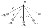 In general \[V=\sum\limits_{i=1}^{X}{\frac{k{{Q}_{i}}}{{{r}_{i}}}}\]
(5) Electric potential due to a continuous charge distribution : The potential due to a continuous charge distribution is the sum of potentials of all the infinitesimal charge elements in which the distribution may be divided i.e.,
\[V=\int{dV},\,\,\,\,=\int{\frac{dQ}{4\pi {{\varepsilon }_{0}}r}}\]
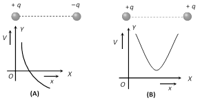
(6) Graphical representation of potential : As we move on the line joining two charges then variation of potential with distance is shown below
In general \[V=\sum\limits_{i=1}^{X}{\frac{k{{Q}_{i}}}{{{r}_{i}}}}\]
(5) Electric potential due to a continuous charge distribution : The potential due to a continuous charge distribution is the sum of potentials of all the infinitesimal charge elements in which the distribution may be divided i.e.,
\[V=\int{dV},\,\,\,\,=\int{\frac{dQ}{4\pi {{\varepsilon }_{0}}r}}\]
(6) Graphical representation of potential : As we move on the line joining two charges then variation of potential with distance is shown below
 (7) Potential difference : In an electric field potential difference between two points A and B is defined as equal to the amount of work done (by external agent) in moving a unit positive charge from point A to point B i.e., \[{{V}_{B}}-{{V}_{A}}=\frac{W}{{{q}_{0}}}\]
 Current Affairs CategoriesArchive
Trending Current Affairs


You need to login to perform this action. |

