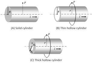
 In all above cases magnetic field outside the wire at \[P\,\,\oint{\overrightarrow{B}.\overrightarrow{dl}={{\mu }_{0}}i}\] \[\Rightarrow \] \[B\int{dl}={{\mu }_{0}}i\]\[\Rightarrow \] \[B\times 2\pi r={{\mu }_{0}}i\]\[\Rightarrow \]\[{{B}_{out}}=\frac{{{\mu }_{0}}i}{2\pi r}\]
In all the above cases \[{{B}_{surface}}=\frac{{{\mu }_{0}}i}{2\pi R}\]
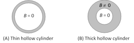
(2) Inside the hollow cylinder : Magnetic field inside the hollow cylinder is zero.
In all above cases magnetic field outside the wire at \[P\,\,\oint{\overrightarrow{B}.\overrightarrow{dl}={{\mu }_{0}}i}\] \[\Rightarrow \] \[B\int{dl}={{\mu }_{0}}i\]\[\Rightarrow \] \[B\times 2\pi r={{\mu }_{0}}i\]\[\Rightarrow \]\[{{B}_{out}}=\frac{{{\mu }_{0}}i}{2\pi r}\]
In all the above cases \[{{B}_{surface}}=\frac{{{\mu }_{0}}i}{2\pi R}\]
(2) Inside the hollow cylinder : Magnetic field inside the hollow cylinder is zero.
 (3) Inside the solid cylinder : Current enclosed by loop \[(i')\] is lesser then the total current \[(i)\]
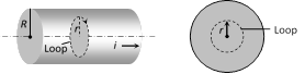 Current density is uniform i.e. \[l=l'\Rightarrow i'=i\times \frac{A'}{A}=i\,\left( \frac{{{r}^{2}}}{{{R}^{2}}} \right)\]
Hence at inside point \[\oint{\overrightarrow{{{B}_{in}}}.\,d\overrightarrow{l\,\,}={{\mu }_{0}}i'}\] \[\Rightarrow \]\[B=\frac{{{\mu }_{0}}}{2\pi }.\frac{ir}{{{R}^{2}}}\]
(4) Inside the thick portion of hollow cylinder : Current enclosed by loop is given as \[i'=i\times \frac{A'}{A}=i\times \frac{({{r}^{2}}-R_{1}^{2})}{(R_{2}^{2}-R_{1}^{2})}\]
Current density is uniform i.e. \[l=l'\Rightarrow i'=i\times \frac{A'}{A}=i\,\left( \frac{{{r}^{2}}}{{{R}^{2}}} \right)\]
Hence at inside point \[\oint{\overrightarrow{{{B}_{in}}}.\,d\overrightarrow{l\,\,}={{\mu }_{0}}i'}\] \[\Rightarrow \]\[B=\frac{{{\mu }_{0}}}{2\pi }.\frac{ir}{{{R}^{2}}}\]
(4) Inside the thick portion of hollow cylinder : Current enclosed by loop is given as \[i'=i\times \frac{A'}{A}=i\times \frac{({{r}^{2}}-R_{1}^{2})}{(R_{2}^{2}-R_{1}^{2})}\]
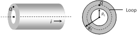 Hence at point Q \[\oint{\overrightarrow{B}.\,d\overrightarrow{l\,\,}={{\mu }_{0}}i'}\]\[\Rightarrow \]\[B=\frac{{{\mu }_{0}}i}{2\pi r}.\frac{({{r}^{2}}-R_{1}^{2})}{(R_{2}^{2}-R_{1}^{2})}\]
 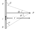 \[B=\frac{{{\mu }_{0}}}{4\pi }.\frac{i}{r}\,(\sin {{\varphi }_{1}}+\sin {{\varphi }_{2}})\]
From figure \[\alpha =({{90}^{o}}-{{\varphi }_{1}})\]
and \[\beta =({{90}^{o}}+{{\varphi }_{2}})\]
Hence \[B=\frac{{{\mu }_{o}}}{4\pi }.\frac{i}{r}(\cos \alpha -\cos \beta )\]
(1) For a wire of finite length : Magnetic field at a point which lies on perpendicular bisector of finite length wire
\[B=\frac{{{\mu }_{0}}}{4\pi }.\frac{i}{r}\,(\sin {{\varphi }_{1}}+\sin {{\varphi }_{2}})\]
From figure \[\alpha =({{90}^{o}}-{{\varphi }_{1}})\]
and \[\beta =({{90}^{o}}+{{\varphi }_{2}})\]
Hence \[B=\frac{{{\mu }_{o}}}{4\pi }.\frac{i}{r}(\cos \alpha -\cos \beta )\]
(1) For a wire of finite length : Magnetic field at a point which lies on perpendicular bisector of finite length wire
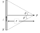 \[{{\varphi }_{1}}={{\varphi }_{2}}=\varphi \]
So \[B=\frac{{{\mu }_{0}}}{4\pi }.\frac{i}{r}(2\sin \varphi )\]
(2) For a wire of infinite length : When the linear conductor XY is of infinite length and the point P lies near the centre of the conductor \[{{\phi }_{1}}={{\phi }_{2}}={{90}^{o}}\].
So,\[B=\frac{{{\mu }_{0}}}{4\pi }\frac{i}{r}[\sin {{90}^{o}}+\sin {{90}^{o}}]\]
\[=\frac{{{\mu }_{0}}}{4\pi }\frac{2i}{r}\]
\[{{\varphi }_{1}}={{\varphi }_{2}}=\varphi \]
So \[B=\frac{{{\mu }_{0}}}{4\pi }.\frac{i}{r}(2\sin \varphi )\]
(2) For a wire of infinite length : When the linear conductor XY is of infinite length and the point P lies near the centre of the conductor \[{{\phi }_{1}}={{\phi }_{2}}={{90}^{o}}\].
So,\[B=\frac{{{\mu }_{0}}}{4\pi }\frac{i}{r}[\sin {{90}^{o}}+\sin {{90}^{o}}]\]
\[=\frac{{{\mu }_{0}}}{4\pi }\frac{2i}{r}\]
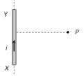 (3) For a wire of semi-infinite length : When the linear conductor is of infinite length and the point P lies near the end Y or X. \[{{\varphi }_{1}}={{90}^{o}}\] and \[{{\varphi }_{2}}={{0}^{o}}\]
So, \[B=\frac{{{\mu }_{0}}}{4\pi }\frac{i}{r}[\sin {{90}^{o}}+\sin {{0}^{o}}]\]
\[=\frac{{{\mu }_{0}}i}{4\pi r}\]
(3) For a wire of semi-infinite length : When the linear conductor is of infinite length and the point P lies near the end Y or X. \[{{\varphi }_{1}}={{90}^{o}}\] and \[{{\varphi }_{2}}={{0}^{o}}\]
So, \[B=\frac{{{\mu }_{0}}}{4\pi }\frac{i}{r}[\sin {{90}^{o}}+\sin {{0}^{o}}]\]
\[=\frac{{{\mu }_{0}}i}{4\pi r}\]
 (4) For axial position of wire : When point P lies on axial position of current carrying conductor then magnetic field at P
| Condition | Figure | Magnetic field | ||||||||||||||||||||||
| Arc subtends angle \[\theta \] at the centre | 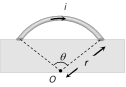 |
\[B=\frac{{{\mu }_{0}}}{4\pi }.\frac{\theta \,i}{r}\] | ||||||||||||||||||||||
| Arc subtends angle \[(2\pi -\theta )\]at the centre | 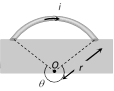 |
\[B=\frac{{{\mu }_{0}}}{4\pi }.\frac{(2\pi -\theta )\,i}{r}\] | ||||||||||||||||||||||
| Semi-circular arc |  |
\[B=\frac{{{\mu }_{0}}}{4\pi }.\frac{\pi i}{r}=\frac{{{\mu }_{0}}i}{4r}\] | ||||||||||||||||||||||
| Three quarter semi-circular current carrying arc |  |
\[B=\frac{{{\mu }_{0}}}{4\pi }.\frac{\left( 2\pi -\frac{\pi }{2} \right)\,i}{r}\] \[=\frac{3{{\mu }_{0}}i}{8r}\] | ||||||||||||||||||||||
| Circular current carrying arc |  |
more...
If a coil of radius \[r,\] carrying current \[i\] then magnetic field on it's axis at a distance \[x\] from its centre given by (Application of Biot-Savart's law)
 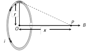 (1) \[{{B}_{axis}}=\frac{{{\mu }_{0}}}{4\pi }.\frac{2\pi Ni{{r}^{2}}}{{{({{x}^{2}}+{{r}^{2}})}^{3/2}}};\] where N = number of turns in coil.
(2) At centre \[x=0\Rightarrow \]\[{{B}_{centre}}=\frac{{{\mu }_{0}}}{4\pi }.\frac{2\pi Ni}{r}\]\[=\frac{{{\mu }_{0}}Ni}{2r}={{B}_{\max }}\]
(3) The ratio of magnetic field at the centre of circular coil and on it's axis is given by \[\frac{{{B}_{centre}}}{{{B}_{axis}}}={{\left( 1+\frac{{{x}^{\mathbf{2}}}}{{{r}^{\mathbf{2}}}} \right)}^{\mathbf{3/2}}}\]
(4) If \[x>>r\Rightarrow \] \[{{B}_{axis}}=\frac{{{\mu }_{0}}}{4\pi }.\frac{2\pi \,Ni{{r}^{2}}}{{{x}^{3}}}=\frac{{{\mu }_{0}}}{4\pi }.\frac{2NiA}{{{x}^{3}}}\]
where \[A=\pi {{r}^{2}}=\] Area of each turn of the coil.
(5) B-x curve : The variation of magnetic field due to a circular coil as the distance x varies as shown in the figure.
B varies non-linearly with distance x as shown in figure and is maximum when \[{{x}^{2}}=\min =0\], i.e., the point is at the centre of the coil and it is zero at \[x=\pm \,\infty \]. .
(1) \[{{B}_{axis}}=\frac{{{\mu }_{0}}}{4\pi }.\frac{2\pi Ni{{r}^{2}}}{{{({{x}^{2}}+{{r}^{2}})}^{3/2}}};\] where N = number of turns in coil.
(2) At centre \[x=0\Rightarrow \]\[{{B}_{centre}}=\frac{{{\mu }_{0}}}{4\pi }.\frac{2\pi Ni}{r}\]\[=\frac{{{\mu }_{0}}Ni}{2r}={{B}_{\max }}\]
(3) The ratio of magnetic field at the centre of circular coil and on it's axis is given by \[\frac{{{B}_{centre}}}{{{B}_{axis}}}={{\left( 1+\frac{{{x}^{\mathbf{2}}}}{{{r}^{\mathbf{2}}}} \right)}^{\mathbf{3/2}}}\]
(4) If \[x>>r\Rightarrow \] \[{{B}_{axis}}=\frac{{{\mu }_{0}}}{4\pi }.\frac{2\pi \,Ni{{r}^{2}}}{{{x}^{3}}}=\frac{{{\mu }_{0}}}{4\pi }.\frac{2NiA}{{{x}^{3}}}\]
where \[A=\pi {{r}^{2}}=\] Area of each turn of the coil.
(5) B-x curve : The variation of magnetic field due to a circular coil as the distance x varies as shown in the figure.
B varies non-linearly with distance x as shown in figure and is maximum when \[{{x}^{2}}=\min =0\], i.e., the point is at the centre of the coil and it is zero at \[x=\pm \,\infty \]. .
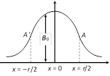 (6) Point of inflection (A and A') : Also known as points of curvature change or points of zero curvature.
(i) At these points B varies linearly with \[x\Rightarrow \frac{dB}{dx}=\] constant \[\Rightarrow \frac{{{d}^{2}}B}{d{{x}^{2}}}=0\].
(ii) These are located at \[x=\pm \frac{r}{2}\] from the centre of the coil and the magnetic field at \[x=\frac{r}{2}\] is \[B=\frac{4{{\mu }_{0}}Ni}{5\sqrt{5}\,r}\]
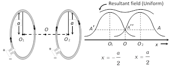
(7) Helmholtz coils
(i) This is the set-up of two coaxial coils of same radius such that distance between their centres is equal to their radius.
(ii) At axial mid point O, magnetic field is given by \[B=\frac{8{{\mu }_{0}}Ni}{5\sqrt{5}R}=0.716\frac{{{\mu }_{0}}Ni}{R}=1.432\,B\], where \[B=\frac{{{\mu }_{0}}Ni}{2R}\]
(iii) Current direction is same in both coils otherwise this arrangement is not called Helmholtz's coil arrangement.
(iv) Number of points of inflextion \[\Rightarrow \] Three \[(A,\,A',\,A'')\]
(6) Point of inflection (A and A') : Also known as points of curvature change or points of zero curvature.
(i) At these points B varies linearly with \[x\Rightarrow \frac{dB}{dx}=\] constant \[\Rightarrow \frac{{{d}^{2}}B}{d{{x}^{2}}}=0\].
(ii) These are located at \[x=\pm \frac{r}{2}\] from the centre of the coil and the magnetic field at \[x=\frac{r}{2}\] is \[B=\frac{4{{\mu }_{0}}Ni}{5\sqrt{5}\,r}\]
(7) Helmholtz coils
(i) This is the set-up of two coaxial coils of same radius such that distance between their centres is equal to their radius.
(ii) At axial mid point O, magnetic field is given by \[B=\frac{8{{\mu }_{0}}Ni}{5\sqrt{5}R}=0.716\frac{{{\mu }_{0}}Ni}{R}=1.432\,B\], where \[B=\frac{{{\mu }_{0}}Ni}{2R}\]
(iii) Current direction is same in both coils otherwise this arrangement is not called Helmholtz's coil arrangement.
(iv) Number of points of inflextion \[\Rightarrow \] Three \[(A,\,A',\,A'')\]
Amperes law gives another method to calculate the magnetic field due to a given current distribution.
Line integral of the magnetic field \[\overrightarrow{B}\] around any closed curve is equal to \[{{\mu }_{0}}\] times the net current i threading through the area enclosed by the curve i.e.
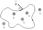 \[\oint{\overrightarrow{B}\cdot \overrightarrow{dI}={{\mu }_{0}}\sum i}={{\mu }_{0}}({{i}_{1}}+{{i}_{3}}-{{i}_{2}})\]
Also using \[\overrightarrow{B}={{\mu }_{0}}\overrightarrow{H}\] (where \[\overrightarrow{H}=\] magnetising field)
\[\oint{{{\mu }_{0}}\overrightarrow{H}.\overrightarrow{dl}}={{\mu }_{0}}\Sigma i\]\[\Rightarrow \]\[\oint{\overrightarrow{H}.\overrightarrow{dl}=\sum i}\]
Total current crossing the above area is \[({{i}_{1}}+{{i}_{3}}-{{i}_{2}})\]. Any current outside the area is not included in net current. (Outward \[\to +ve\], Inward \[\to -ve\])
Biot-Savart's law v/s Ampere's law
\[\oint{\overrightarrow{B}\cdot \overrightarrow{dI}={{\mu }_{0}}\sum i}={{\mu }_{0}}({{i}_{1}}+{{i}_{3}}-{{i}_{2}})\]
Also using \[\overrightarrow{B}={{\mu }_{0}}\overrightarrow{H}\] (where \[\overrightarrow{H}=\] magnetising field)
\[\oint{{{\mu }_{0}}\overrightarrow{H}.\overrightarrow{dl}}={{\mu }_{0}}\Sigma i\]\[\Rightarrow \]\[\oint{\overrightarrow{H}.\overrightarrow{dl}=\sum i}\]
Total current crossing the above area is \[({{i}_{1}}+{{i}_{3}}-{{i}_{2}})\]. Any current outside the area is not included in net current. (Outward \[\to +ve\], Inward \[\to -ve\])
Biot-Savart's law v/s Ampere's law
If magnetic field is directed perpendicular and into the plane of the paper it is represented by Ä (cross) while if magnetic field is directed perpendicular and out of the plane of the paper it is represented by (dot)
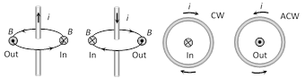 In : Magnetic field is away from the observer or perpendicular inwards.
Out : Magnetic field is towards the observer or perpendicular outwards.
In : Magnetic field is away from the observer or perpendicular inwards.
Out : Magnetic field is towards the observer or perpendicular outwards.
The direction of magnetic field is determined with the help of the following simple laws :
(1) Maxwell's cork screw rule : According to this rule, if we imagine a right handed screw placed along the current carrying linear conductor, be rotated such that the screw moves in the direction of flow of current, then the direction of rotation of the thumb gives the direction of magnetic lines of force.
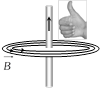
 (2) Right hand thumb rule : According to this rule if a straight current carrying conductor is held in the right hand such that the thumb of the hand represents the direction of current flow, then the direction of folding fingers will represent the direction of magnetic lines of force.
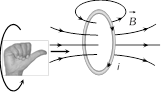
 (3) Right hand thumb rule of circular currents : According to this rule if the direction of current in circular conducting coil is in the direction of folding fingers of right hand, then the direction of magnetic field will be in the direction of stretched thumb.
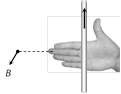
 (4) Right hand palm rule : If we stretch our right hand such that fingers point towards the point. At which magnetic field is required while thumb is in the direction of current then normal to the palm will show the direction of magnetic field.
Biot-Savart's law is used to determine the magnetic field at any point due to a current carrying conductor.
This law is although for infinitesimally small conductor yet it can be used for long conductors. In order to understand the Biot-Savart's law, we need to understand the term current-element.
Current element It is the product of current and length of infinitesimal segment of current carrying wire.
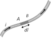 The current element is taken as a vector quantity. Its direction is same as the direction of current. Current element \[AB=i\vec{d}l\]
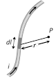
According to Biot-Savart Law, magnetic field at point 'P' due to the current element \[i\vec{d}l\] is given by the expression, \[d\vec{B}=k\frac{i\,dl\sin \theta }{{{r}^{2}}}\hat{n}\] . Also \[\vec{B}=fd\vec{B}=\frac{{{\mu }_{0}}i}{4\pi }.\,\int_{{}}^{{}}{\frac{dl\sin \theta }{{{r}^{2}}}}\hat{n}\]
In C.G.S. k = 1 and in S.I. \[k=\frac{{{\mu }_{0}}}{4\pi }\]
where \[{{\mu }_{0}}=\] Absolute permeability of air or vacuum \[=4\pi \times {{10}^{-7}}\,\frac{Wb}{Amp-metre}\] . It's other units are
\[\frac{henry}{metre}\]or \[\frac{N}{Am{{p}^{2}}}\] or \[\frac{Tesla-metre}{Ampere}\]
vectorially, \[d\vec{B}=\frac{{{\mu }_{0}}}{4\pi }.\frac{i(\vec{d}l\times \hat{r})}{{{r}^{2}}}=\frac{{{\mu }_{0}}}{4\pi }.\frac{i(\vec{d}l\times \vec{r})}{{{r}^{3}}}\]
i.e., \[\vec{B}\] is perpendicular to both \[I\,\vec{d}\,l\] and
\[\vec{r}\]
.
The current element is taken as a vector quantity. Its direction is same as the direction of current. Current element \[AB=i\vec{d}l\]
According to Biot-Savart Law, magnetic field at point 'P' due to the current element \[i\vec{d}l\] is given by the expression, \[d\vec{B}=k\frac{i\,dl\sin \theta }{{{r}^{2}}}\hat{n}\] . Also \[\vec{B}=fd\vec{B}=\frac{{{\mu }_{0}}i}{4\pi }.\,\int_{{}}^{{}}{\frac{dl\sin \theta }{{{r}^{2}}}}\hat{n}\]
In C.G.S. k = 1 and in S.I. \[k=\frac{{{\mu }_{0}}}{4\pi }\]
where \[{{\mu }_{0}}=\] Absolute permeability of air or vacuum \[=4\pi \times {{10}^{-7}}\,\frac{Wb}{Amp-metre}\] . It's other units are
\[\frac{henry}{metre}\]or \[\frac{N}{Am{{p}^{2}}}\] or \[\frac{Tesla-metre}{Ampere}\]
vectorially, \[d\vec{B}=\frac{{{\mu }_{0}}}{4\pi }.\frac{i(\vec{d}l\times \hat{r})}{{{r}^{2}}}=\frac{{{\mu }_{0}}}{4\pi }.\frac{i(\vec{d}l\times \vec{r})}{{{r}^{3}}}\]
i.e., \[\vec{B}\] is perpendicular to both \[I\,\vec{d}\,l\] and
\[\vec{r}\]
.
(1) To measure temperature : A thermocouple is used to measure very high \[({{20000}^{o}}C)\] as well as very low \[(-{{200}^{o}}C)\]temperature in industries and laboratories. The thermocouple used to measure very high temperature is called pyrometer.
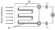
(2) To detect heat radiation : A thermopile is a sensitive instrument used for detection of heat radiation and measurement of their intensity. It is based upon Seebeck effect.
A thermoppile consists of a number of thermocouples of Sb-Bi, all connected in series.
 Heating effect and Thermo-electric effects
|


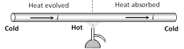
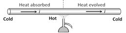 (ii) Negative Thomson's effect : In the elements which show negative Thomson's effect, it is found that the hot end is at low potential and the cold end is at higher potential. Heat is evolved when current is passed from colder end to the hotter end and heat is absorbed when current flows from hotter end to colder end. The metals which shows negative. Thomson's effect are Fe, Co, Bi, Pt, Hg ... etc.
 Thomson's co-efficient : In Thomson's effect it is found that heat released or absorbed is proportional to \[Q\Delta \theta \] i.e. \[H\propto Q\Delta \theta \]\[\Rightarrow \]\[H=\sigma Q\Delta \theta \] where \[\sigma =\] Thomson's coefficient. It's unit is Joule/coulomb\[^{o}C\] or volt/\[^{o}C\] and \[\Delta \theta =\]temperature difference.
If \[Q=1\] and \[\Delta \theta =1\] then \[\sigma =H\] so the amount of heat energy absorbed or evolved per second between two points of a conductor having a unit temperature difference, when a unit current is passed is known as Thomson's co-efficient for the material of a conductor.
It can be proved that Thomson co-efficient of the material of conductor \[\sigma =-T\frac{{{d}^{2}}E}{d{{T}^{2}}}\]\[=-T\left( \frac{dS}{dT} \right)=T\times \beta \]; where \[\beta =\] Thermo electric constant \[=\frac{dS}{dt}\]
Thomson's co-efficient : In Thomson's effect it is found that heat released or absorbed is proportional to \[Q\Delta \theta \] i.e. \[H\propto Q\Delta \theta \]\[\Rightarrow \]\[H=\sigma Q\Delta \theta \] where \[\sigma =\] Thomson's coefficient. It's unit is Joule/coulomb\[^{o}C\] or volt/\[^{o}C\] and \[\Delta \theta =\]temperature difference.
If \[Q=1\] and \[\Delta \theta =1\] then \[\sigma =H\] so the amount of heat energy absorbed or evolved per second between two points of a conductor having a unit temperature difference, when a unit current is passed is known as Thomson's co-efficient for the material of a conductor.
It can be proved that Thomson co-efficient of the material of conductor \[\sigma =-T\frac{{{d}^{2}}E}{d{{T}^{2}}}\]\[=-T\left( \frac{dS}{dT} \right)=T\times \beta \]; where \[\beta =\] Thermo electric constant \[=\frac{dS}{dt}\] 


