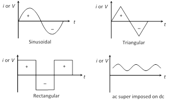
 (3) Equation for i and V : Alternating current or voltage varying as sine function can be written as
\[i={{i}_{0}}\,\sin \omega t={{i}_{0}}\sin \,2\pi vt={{i}_{0}}\sin \frac{2\pi }{T}t\]
and \[V={{V}_{0}}\sin \omega t={{V}_{0}}\sin 2\pi \nu t={{V}_{0}}\sin \frac{2\pi }{T}t\]
(3) Equation for i and V : Alternating current or voltage varying as sine function can be written as
\[i={{i}_{0}}\,\sin \omega t={{i}_{0}}\sin \,2\pi vt={{i}_{0}}\sin \frac{2\pi }{T}t\]
and \[V={{V}_{0}}\sin \omega t={{V}_{0}}\sin 2\pi \nu t={{V}_{0}}\sin \frac{2\pi }{T}t\]
 where \[i\] and \[V\] are Instantaneous values of current and voltage,
\[{{i}_{0}}\] and \[{{V}_{0}}\] are peak values of current and voltage
\[\omega =\] Angular frequency in rad/sec, \[v=\] Frequency in Hz and \[T=\]time period
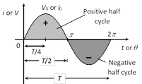
(i) The time taken to complete one cycle of variations is called the periodic time or time period.
(ii) Alternating quantity is positive for half the cycle and negative for the rest half. Hence average value of alternating quantity (i or V) over a complete cycle is zero.
(iii) The value of alternating quantity is zero or maximum \[2v\] times every second. The direction also changes \[2v\] times every second.
(iv) Generally sinusoidal waveform is used as alternating current/voltage.
(v) At \[t=\frac{T}{4}\] from the beginning, i or V reaches to their maximum value.
where \[i\] and \[V\] are Instantaneous values of current and voltage,
\[{{i}_{0}}\] and \[{{V}_{0}}\] are peak values of current and voltage
\[\omega =\] Angular frequency in rad/sec, \[v=\] Frequency in Hz and \[T=\]time period
(i) The time taken to complete one cycle of variations is called the periodic time or time period.
(ii) Alternating quantity is positive for half the cycle and negative for the rest half. Hence average value of alternating quantity (i or V) over a complete cycle is zero.
(iii) The value of alternating quantity is zero or maximum \[2v\] times every second. The direction also changes \[2v\] times every second.
(iv) Generally sinusoidal waveform is used as alternating current/voltage.
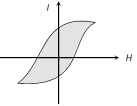
(v) At \[t=\frac{T}{4}\] from the beginning, i or V reaches to their maximum value. 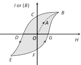 The lack of retracibility as
shown in figure is called hysteresis and the curve is known as hysteresis loop.
(1) Retentivity : When H is reduced, I reduces but
is not zero when \[H=0\]. The remainder value OC of magnetisation when \[H=0\]
is called the residual magnetism or retentivity.
The property by virtue of
which the magnetism (I) remains in a material even on the removal of
magnetising field is called Retentivity or Residual magnetism.
(2) Corecivity or
corecive force : When magnetic field H is reversed, the
magnetisation decreases and for a particular value of H, denoted by \[{{H}_{c}}\],
it becomes zero i.e., \[{{H}_{c}}=OD\] when \[l=0\]. This value of H
is called the corecivity.
Magnetic hard substance
(steel) \[\to \] High corecvity
Magnetic soft substance
(soft iron) \[\to \]Low corecivity
(3) When field H is
further increased in reverse direction, the intensity of magnetisation attains
saturation value in reverse direction (i.e. point E)
(4) When H is
decreased to zero and changed direction in steps, we get the part EFGB.
Thus complete cycle of
magnetisation and demagnetisation is represented by BCDEFGB. This curve
is known as hysteresis curve
Comparison
between soft iron and steel
The lack of retracibility as
shown in figure is called hysteresis and the curve is known as hysteresis loop.
(1) Retentivity : When H is reduced, I reduces but
is not zero when \[H=0\]. The remainder value OC of magnetisation when \[H=0\]
is called the residual magnetism or retentivity.
The property by virtue of
which the magnetism (I) remains in a material even on the removal of
magnetising field is called Retentivity or Residual magnetism.
(2) Corecivity or
corecive force : When magnetic field H is reversed, the
magnetisation decreases and for a particular value of H, denoted by \[{{H}_{c}}\],
it becomes zero i.e., \[{{H}_{c}}=OD\] when \[l=0\]. This value of H
is called the corecivity.
Magnetic hard substance
(steel) \[\to \] High corecvity
Magnetic soft substance
(soft iron) \[\to \]Low corecivity
(3) When field H is
further increased in reverse direction, the intensity of magnetisation attains
saturation value in reverse direction (i.e. point E)
(4) When H is
decreased to zero and changed direction in steps, we get the part EFGB.
Thus complete cycle of
magnetisation and demagnetisation is represented by BCDEFGB. This curve
is known as hysteresis curve
Comparison
between soft iron and steel
| Soft iron | Steel |
|
|
| The area of hysteresis loop is less (low energy loss) | The area of hysteresis loop is large (high energy loss) |
| Less relativity and corecive force | More retentivity and corecive force |
| Magnetic permeability is high | Magnetic permeability is less |
| I and \[\chi \] both are high | I and \[\chi \] both are low |
| It magnetised and demagnetised easily | Magnetisation and demagnetisation is not easy |
|
Used in dynamo, transformer, electromagnet tape more...
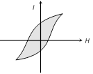
On the basis of mutual interactions or
behaviour of various materials in an external magnetic field, the materials are
divided in three main categories.
(1) Diamagnetic materials :
Diamagnetism is the intrinsic property of every material and it is generated
due to mutual interaction between the applied magnetic field and orbital motion
of electrons.
(2) Paramagnetic materials : In
these substances the inner orbits of atoms are incomplete. The electron spins
are uncoupled, consequently on applying a magnetic field the magnetic moment
generated due to spin motion align in the direction of magnetic field and
induces magnetic moment in its direction due to which the material gets feebly
magnetised. In these materials the electron number is odd.
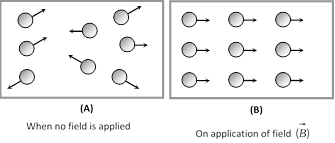 (3) Ferromagnetic
materials : In some materials, the permanent atomic magnetic moments have
strong tendency to align themselves even without any external field.
These materials are
called ferromagnetic materials.
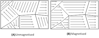
In every unmagnetised
ferromagnetic material, the atoms form domains inside the material. Different
domains, however, have different directions of magnetic moment and hence the
materials remain unmagnetised. On applying an external magnetic field, these
domains rotate and align in the direction of magnetic field.
(3) Ferromagnetic
materials : In some materials, the permanent atomic magnetic moments have
strong tendency to align themselves even without any external field.
These materials are
called ferromagnetic materials.
In every unmagnetised
ferromagnetic material, the atoms form domains inside the material. Different
domains, however, have different directions of magnetic moment and hence the
materials remain unmagnetised. On applying an external magnetic field, these
domains rotate and align in the direction of magnetic field.
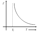
 (4) Curie Law : The magnetic
susceptibility of paramagnetic substances is inversely proportional to its
absolute temperature i.e. \[\chi \propto \frac{1}{T}\]\[\Rightarrow \]\[\chi
\propto \frac{C}{T}\]; where C = Curie constant, T = absolute
temperature.
On increasing temperature, the magnetic
susceptibility of paramagnetic materials decreases and vice versa.
The magnetic susceptibility of
ferromagnetic substances does not change according to Curie law.
(5) Curie temperature \[({{T}_{c}})\] :
The temperature above which a ferromagnetic material behaves like a
paramagnetic material is defined as Curie temperature \[({{T}_{c}})\].
or
The minimum temperature at which a
ferromagnetic substance is converted into paramagnetic substance is defined as
Curie temperature. For various ferromagnetic materials its values are
different, e.g. for Ni, \[{{T}_{{{C}_{Ni}}}}={{358}^{o}}C\]for Fe,
\[{{T}_{{{C}_{Fe}}}}={{770}^{o}}C\]
for CO, \[{{T}_{{{C}_{CO}}}}={{1120}^{o}}C\]
At this temperature the ferromagnetism of
the substances suddenly vanishes.
(6) Curie-weiss law : At temperatures
above Curie temperature the magnetic susceptibility of ferromagnetic materials
is inversely proportional to \[(T-{{T}_{c}})\]
(4) Curie Law : The magnetic
susceptibility of paramagnetic substances is inversely proportional to its
absolute temperature i.e. \[\chi \propto \frac{1}{T}\]\[\Rightarrow \]\[\chi
\propto \frac{C}{T}\]; where C = Curie constant, T = absolute
temperature.
On increasing temperature, the magnetic
susceptibility of paramagnetic materials decreases and vice versa.
The magnetic susceptibility of
ferromagnetic substances does not change according to Curie law.
(5) Curie temperature \[({{T}_{c}})\] :
The temperature above which a ferromagnetic material behaves like a
paramagnetic material is defined as Curie temperature \[({{T}_{c}})\].
or
The minimum temperature at which a
ferromagnetic substance is converted into paramagnetic substance is defined as
Curie temperature. For various ferromagnetic materials its values are
different, e.g. for Ni, \[{{T}_{{{C}_{Ni}}}}={{358}^{o}}C\]for Fe,
\[{{T}_{{{C}_{Fe}}}}={{770}^{o}}C\]
for CO, \[{{T}_{{{C}_{CO}}}}={{1120}^{o}}C\]
At this temperature the ferromagnetism of
the substances suddenly vanishes.
(6) Curie-weiss law : At temperatures
above Curie temperature the magnetic susceptibility of ferromagnetic materials
is inversely proportional to \[(T-{{T}_{c}})\]
 i.e. \[\chi \propto
\frac{1}{T-{{T}_{c}}}\]
\[\Rightarrow \] \[\chi
=\frac{C}{(T-{{T}_{c}})}\]
Here \[{{T}_{c}}=\] Curie
temperature
\[\chi -T\] curve
is shown (for Curie-Weiss Law)
i.e. \[\chi \propto
\frac{1}{T-{{T}_{c}}}\]
\[\Rightarrow \] \[\chi
=\frac{C}{(T-{{T}_{c}})}\]
Here \[{{T}_{c}}=\] Curie
temperature
\[\chi -T\] curve
is shown (for Curie-Weiss Law)
Vibration magnetometer is used for comparison of magnetic moments and magnetic fields. This device works on the principle, that whenever a freely suspended magnet in a uniform magnetic field, is disturbed from it's equilibrium position, it starts vibrating about the mean position.
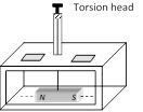 Time period of oscillation of experimental bar magnet (magnetic moment M) in earth's magnetic field \[({{B}_{H}})\] is given by the formula. \[T=2\pi \sqrt{\frac{I}{M{{B}_{H}}}}\]; where, \[I=\] moment of inertia of short bar magnet \[=\frac{w{{L}^{2}}}{12}\] (w = mass of bar magnet)
(1) Determination of magnetic moment of a magnet : The experimental (given) magnet is put into vibration magnetometer and it's time period T is determined. Now \[T=2\pi \sqrt{\frac{I}{M{{B}_{H}}}}\,\,\Rightarrow \,M=\frac{4{{\pi }^{2}}I}{{{B}_{H}}.{{T}^{2}}}\]
(2) Comparison of horizontal components of earth's magnetic field at two places
\[T=2\pi \sqrt{\frac{I}{M{{B}_{H}}}}\] ; since I and M of the magnet are constant,
So \[{{T}^{2}}\propto \frac{1}{{{B}_{H}}}\,\,\Rightarrow \,\,\frac{{{({{B}_{H}})}_{1}}}{{{({{B}_{H}})}_{2}}}=\frac{T_{2}^{2}}{T_{1}^{2}}\]
(3) Comparison of magnetic moment of two magnets of same size and mass
\[T=2\pi \sqrt{\frac{I}{M.{{B}_{H}}}}\] ; Here I and BH are constants.
So \[M\propto \frac{1}{{{T}^{2}}}\] \[\Rightarrow \]\[\frac{{{M}_{1}}}{{{M}_{2}}}=\frac{T_{2}^{2}}{T_{1}^{2}}\]
(4) Comparison of magnetic moments by sum and difference method
Sum position
Net magnetic moment
\[{{M}_{s}}={{M}_{1}}+{{M}_{2}}\]
Net moment of inertia \[{{l}_{s}}={{l}_{1}}+{{l}_{2}}\]
Time period of oscillation of this pair in earth's magnetic field \[({{B}_{H}})\]
Time period of oscillation of experimental bar magnet (magnetic moment M) in earth's magnetic field \[({{B}_{H}})\] is given by the formula. \[T=2\pi \sqrt{\frac{I}{M{{B}_{H}}}}\]; where, \[I=\] moment of inertia of short bar magnet \[=\frac{w{{L}^{2}}}{12}\] (w = mass of bar magnet)
(1) Determination of magnetic moment of a magnet : The experimental (given) magnet is put into vibration magnetometer and it's time period T is determined. Now \[T=2\pi \sqrt{\frac{I}{M{{B}_{H}}}}\,\,\Rightarrow \,M=\frac{4{{\pi }^{2}}I}{{{B}_{H}}.{{T}^{2}}}\]
(2) Comparison of horizontal components of earth's magnetic field at two places
\[T=2\pi \sqrt{\frac{I}{M{{B}_{H}}}}\] ; since I and M of the magnet are constant,
So \[{{T}^{2}}\propto \frac{1}{{{B}_{H}}}\,\,\Rightarrow \,\,\frac{{{({{B}_{H}})}_{1}}}{{{({{B}_{H}})}_{2}}}=\frac{T_{2}^{2}}{T_{1}^{2}}\]
(3) Comparison of magnetic moment of two magnets of same size and mass
\[T=2\pi \sqrt{\frac{I}{M.{{B}_{H}}}}\] ; Here I and BH are constants.
So \[M\propto \frac{1}{{{T}^{2}}}\] \[\Rightarrow \]\[\frac{{{M}_{1}}}{{{M}_{2}}}=\frac{T_{2}^{2}}{T_{1}^{2}}\]
(4) Comparison of magnetic moments by sum and difference method
Sum position
Net magnetic moment
\[{{M}_{s}}={{M}_{1}}+{{M}_{2}}\]
Net moment of inertia \[{{l}_{s}}={{l}_{1}}+{{l}_{2}}\]
Time period of oscillation of this pair in earth's magnetic field \[({{B}_{H}})\]
 \[T=2\pi \sqrt{\frac{I}{M\,{{B}_{H}}}}\]
and frequency \[\nu =\frac{1}{2\pi }\sqrt{\frac{M\,{{B}_{H}}}{I}}\]
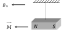
Now a secondary magnet placed near the primary magnet so primary magnet oscillate in a new field with is the resultant of B and BH and now time period, is noted again.
\[T=2\pi \sqrt{\frac{I}{M\,{{B}_{H}}}}\]
and frequency \[\nu =\frac{1}{2\pi }\sqrt{\frac{M\,{{B}_{H}}}{I}}\]
Now a secondary magnet placed near the primary magnet so primary magnet oscillate in a new field with is the resultant of B and BH and now time period, is noted again.
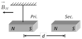 \[T'=2\pi \sqrt{\frac{I}{M(B+{{B}_{H}})}}\]
or \[\nu \,'=\frac{1}{2\pi }\sqrt{\frac{M(B+{{B}_{H}})}{I}}\]
\[\Rightarrow \]\[\frac{B}{{{B}_{H}}}={{\left( \frac{\nu \,'}{\nu } \right)}^{2}}-1\]
\[T'=2\pi \sqrt{\frac{I}{M(B+{{B}_{H}})}}\]
or \[\nu \,'=\frac{1}{2\pi }\sqrt{\frac{M(B+{{B}_{H}})}{I}}\]
\[\Rightarrow \]\[\frac{B}{{{B}_{H}}}={{\left( \frac{\nu \,'}{\nu } \right)}^{2}}-1\]
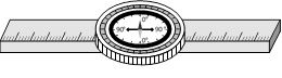
It's working is based on the principle of tangent law. It consists of a small compass needle, pivoted at the centre of a circular box. The box is kept in a wooden frame having two meter scale fitted on it's two arms. Reading of a scale at any point directly gives the distance of that point from the centre of compass needle.
 (1) Tan A position : In this position the magnetometer is set perpendicular to magnetic meridian. So that, magnetic field due to magnet, is in axial position and perpendicular to earth's field. Hence \[{{B}_{H}}\tan \theta =\frac{{{\mu }_{0}}}{4\pi }.\frac{2Mr}{{{({{r}^{2}}-{{l}^{2}})}^{2}}}\] or \[{{B}_{H}}\tan \theta =\frac{{{\mu }_{0}}}{4\pi }.\frac{2M}{{{r}^{3}}}\]
(2) Tan B position : The arms of magnetometer are set in magnetic meridian, so that the magnetic field due to magnet is at it's equatorial position. Hence \[{{B}_{H}}\tan \theta =\frac{{{\mu }_{0}}}{4\pi }.\frac{M}{{{({{r}^{2}}+{{l}^{2}})}^{3/2}}}\] or \[{{B}_{H}}\tan \theta =\frac{{{\mu }_{0}}}{4\pi }.\frac{M}{{{r}^{3}}}\]
(3) Comparison of magnetic moments : According to deflection method \[\frac{{{M}_{1}}}{{{M}_{2}}}=\frac{\tan {{\theta }_{1}}}{\tan {{\theta }_{2}}}\]
According to null deflection method \[\frac{{{M}_{1}}}{{{M}_{2}}}={{\left( \frac{{{d}_{1}}}{{{d}_{2}}} \right)}^{3}}\]
(1) Tan A position : In this position the magnetometer is set perpendicular to magnetic meridian. So that, magnetic field due to magnet, is in axial position and perpendicular to earth's field. Hence \[{{B}_{H}}\tan \theta =\frac{{{\mu }_{0}}}{4\pi }.\frac{2Mr}{{{({{r}^{2}}-{{l}^{2}})}^{2}}}\] or \[{{B}_{H}}\tan \theta =\frac{{{\mu }_{0}}}{4\pi }.\frac{2M}{{{r}^{3}}}\]
(2) Tan B position : The arms of magnetometer are set in magnetic meridian, so that the magnetic field due to magnet is at it's equatorial position. Hence \[{{B}_{H}}\tan \theta =\frac{{{\mu }_{0}}}{4\pi }.\frac{M}{{{({{r}^{2}}+{{l}^{2}})}^{3/2}}}\] or \[{{B}_{H}}\tan \theta =\frac{{{\mu }_{0}}}{4\pi }.\frac{M}{{{r}^{3}}}\]
(3) Comparison of magnetic moments : According to deflection method \[\frac{{{M}_{1}}}{{{M}_{2}}}=\frac{\tan {{\theta }_{1}}}{\tan {{\theta }_{2}}}\]
According to null deflection method \[\frac{{{M}_{1}}}{{{M}_{2}}}={{\left( \frac{{{d}_{1}}}{{{d}_{2}}} \right)}^{3}}\]
It consists of three circular coils of insulated copper wire wound on a vertical circular frame made of nonmagnetic material as ebonite or wood. A small magnetic compass needle is pivoted at the centre of the vertical circular frame. When the coil of the tangent galvanometer is kept in magnetic meridian and current passes through any of the coil then the needle at the centre gets deflected and comes to an equilibrium position under the action of two perpendicular field : one due to horizontal component of earth and the other due to field (B) set up by the coil due to current.
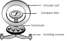 In equilibrium \[B={{B}_{H}}tan\theta \] where \[B=\frac{{{\mu }_{0}}ni}{2r}\]; n = number of turns, r = radius of coil, i = the current to be measured, \[\theta =\] angle made by needle from the direction of \[{{B}_{H}}\] in equilibrium.
Hence \[\frac{{{\mu }_{0}}Ni}{2r}={{B}_{H}}\tan \theta \] \[\Rightarrow \] \[i=k\tan \theta \] where \[k=\frac{2r{{B}_{H}}}{{{\mu }_{0}}N}\] is called reduction factor.
In equilibrium \[B={{B}_{H}}tan\theta \] where \[B=\frac{{{\mu }_{0}}ni}{2r}\]; n = number of turns, r = radius of coil, i = the current to be measured, \[\theta =\] angle made by needle from the direction of \[{{B}_{H}}\] in equilibrium.
Hence \[\frac{{{\mu }_{0}}Ni}{2r}={{B}_{H}}\tan \theta \] \[\Rightarrow \] \[i=k\tan \theta \] where \[k=\frac{2r{{B}_{H}}}{{{\mu }_{0}}N}\] is called reduction factor.
When a small magnet is suspended in two uniform magnetic fields \[B\] and \[{{B}_{H}}\]which are at right angles to each other, the magnet comes to rest at an angle \[\theta \] with respect to \[{{B}_{H}}\].
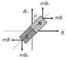 In equilibrium
\[M{{B}_{H}}\sin \theta \]\[=MB\sin \,({{90}^{o}}-\theta )\]
\[\Rightarrow \] \[B={{B}_{H}}\tan \theta .\] This is called tangent law.
In equilibrium
\[M{{B}_{H}}\sin \theta \]\[=MB\sin \,({{90}^{o}}-\theta )\]
\[\Rightarrow \] \[B={{B}_{H}}\tan \theta .\] This is called tangent law.
(1) Magnetic maps : Magnetic maps (i.e. Declination, dip and horizontal component) over the earth vary in magnitude from place to place. It is found that many places have the same value of magnetic elements. The lines are drawn joining all place on the earth having same value of a magnetic element. These lines form magnetic map.
(i) Isogonic lines: These are the lines on the magnetic map joining the places of equal declination.
(ii) Agonic line: The line which passes through places having zero declination is called agonic line.
(iii) Isoclinic lines : These are the lines joining the points of equal dip or inclination.
(iv) Aclinic line : The line joining places of zero dip is called aclinic line (or magnetic equator)
(v) Isodynamic lines : The lines joining the points or places having the same value of horizontal component of earth's magnetic field are called isodynamic lines.
(2) Neutral points : A neutral point is a point at which the resultant magnetic field is zero. In general the neutral point is obtained when horizontal component of earth's field is balanced by the field produced by the magnet.
The magnitude and direction of the magnetic field of the earth at a place are completely given by certain. quantities known as magnetic elements.
(1) Magnetic Declination \[(\theta )\]: It is the angle between geographic and the magnetic meridian planes.
 Declination at a place is expressed at \[{{\theta }^{o}}E\] or \[{{\theta }^{o}}W\] depending upon whether the north pole of the compass needle lies to the east or to the west of the geographical axis.
(2) Angle of inclination or Dip \[(\phi )\] : It is the angle between the direction of intensity of total magnetic field of earth and a horizontal line in the magnetic meridian.
(3) Horizontal component of earth's magnetic field \[({{B}_{H}})\] : Earth's magnetic field is horizontal only at the magnetic equator. At any other place, the total intensity can be resolved into horizontal component \[({{B}_{H}})\] and vertical component \[({{B}_{V}})\].
Also \[{{B}_{H}}=B\cos \phi \] ...... (i) and \[{{B}_{V}}=B\sin \varphi \] ...... (ii)
By squaring and adding equation (i) and (ii) \[B=\sqrt{{{B}_{{{H}^{2}}}}+{{B}_{{{V}^{2}}}}}\]
Dividing equation (ii) by equation (i) \[\tan \varphi =\frac{{{B}_{V}}}{{{B}_{H}}}\]
Declination at a place is expressed at \[{{\theta }^{o}}E\] or \[{{\theta }^{o}}W\] depending upon whether the north pole of the compass needle lies to the east or to the west of the geographical axis.
(2) Angle of inclination or Dip \[(\phi )\] : It is the angle between the direction of intensity of total magnetic field of earth and a horizontal line in the magnetic meridian.
(3) Horizontal component of earth's magnetic field \[({{B}_{H}})\] : Earth's magnetic field is horizontal only at the magnetic equator. At any other place, the total intensity can be resolved into horizontal component \[({{B}_{H}})\] and vertical component \[({{B}_{V}})\].
Also \[{{B}_{H}}=B\cos \phi \] ...... (i) and \[{{B}_{V}}=B\sin \varphi \] ...... (ii)
By squaring and adding equation (i) and (ii) \[B=\sqrt{{{B}_{{{H}^{2}}}}+{{B}_{{{V}^{2}}}}}\]
Dividing equation (ii) by equation (i) \[\tan \varphi =\frac{{{B}_{V}}}{{{B}_{H}}}\] Current Affairs CategoriesArchive
Trending Current Affairs


You need to login to perform this action. |

